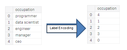
{"metadata":{"kernelspec":{"language":"python","display_name":"Python 3","name":"python3"},"language_info":{"pygments_lexer":"ipython3","nbconvert_exporter":"python","version":"3.6.4","file_extension":".py","codemirror_mode":{"name":"ipython","version":3},"name":"python","mimetype":"text/x-python"}},"nbformat_minor":4,"nbformat":4,"cells":[{"cell_type":"markdown","source":"## ASHRAE - Great Energy Predictor III\n___\n\nThankfully, significant investments are being made to improve building efficiencies to reduce costs and emissions. The question is, are the improvements working? That’s where you come in. Under pay-for-performance financing, the building owner makes payments based on the difference between their real energy consumption and what they would have used without any retrofits. The latter values have to come from a model. Current methods of estimation are fragmented and do not scale well. Some assume a specific meter type or don’t work with different building types.\n\nIn this competition, you’ll develop accurate models of metered building energy usage in the following areas: chilled water, electric, hot water, and steam meters. The data comes from over 1,000 buildings over a three-year timeframe. With better estimates of these energy-saving investments, large scale investors and financial institutions will be more inclined to invest in this area to enable progress in building efficiencies.\n\nFrom the competition page\n\nThis notebook is inspired by Crislânio Macêdo notebook, https://www.kaggle.com/caesarlupum/ashrae-start-here-a-gentle-introduction\n\n\nAnd the competition links is here : https://www.kaggle.com/c/ashrae-energy-prediction","metadata":{}},{"cell_type":"markdown","source":"# <a id='1'>1. Introduction: ASHRAE - Great Energy Predictor III</a>","metadata":{}},{"cell_type":"code","source":"# Suppress warnings \nimport warnings\nwarnings.filterwarnings(\"ignore\", category=DeprecationWarning)\nwarnings.filterwarnings(\"ignore\", category=UserWarning)\nwarnings.filterwarnings(\"ignore\", category=FutureWarning)\nfrom IPython.display import HTML\n","metadata":{"_kg_hide-input":true,"execution":{"iopub.status.busy":"2022-03-28T19:36:19.256625Z","iopub.execute_input":"2022-03-28T19:36:19.256895Z","iopub.status.idle":"2022-03-28T19:36:19.26274Z","shell.execute_reply.started":"2022-03-28T19:36:19.256866Z","shell.execute_reply":"2022-03-28T19:36:19.261621Z"},"trusted":true},"execution_count":null,"outputs":[]},{"cell_type":"markdown","source":"\n## <a id='1-1'>1.1 Data</a>\n","metadata":{}},{"cell_type":"markdown","source":"### Files\n> #### train.csv\n- building_id - Foreign key for the building metadata.\n- meter - The meter id code. Read as {0: electricity, 1: chilledwater, 2: steam, hotwater: 3}. Not every building has all meter types.\n- timestamp - When the measurement was taken\n- meter_reading - The target variable. Energy consumption in kWh (or equivalent). Note that this is real data with measurement error, which we expect will impose a baseline level of modeling error.\n> #### building_meta.csv\n- site_id - Foreign key for the weather files.\n- building_id - Foreign key for training.csv\n- primary_use - Indicator of the primary category of activities for the building based on [EnergyStar](https://www.energystar.gov/buildings/facility-owners-and-managers/existing-buildings/use-portfolio-manager/identify-your-property-type) property type definitions\n- square_feet - Gross floor area of the building\n- year_built - Year building was opened\n- floor_count - Number of floors of the building\n> #### weather_[train/test].csv\nWeather data from a meteorological station as close as possible to the site.\n\n- site_id\n- air_temperature - Degrees Celsius\n- cloud_coverage - Portion of the sky covered in clouds, in [oktas](https://en.wikipedia.org/wiki/Okta)\n- dew_temperature - Degrees Celsius\n- precip_depth_1_hr - Millimeters\n- sea_level_pressure - Millibar/hectopascals\n- wind_direction - Compass direction (0-360)\n- wind_speed - Meters per second\n> #### test.csv\nThe submission files use row numbers for ID codes in order to save space on the file uploads. test.csv has no feature data; it exists so you can get your predictions into the correct order.\n\nrow_id - Row id for your submission file\n- building_id - Building id code\n- meter - The meter id code\n- timestamp - Timestamps for the test data period\n> ####  sample_submission.csv\nA valid sample submission.\n\n","metadata":{}},{"cell_type":"markdown","source":"# <a id='2'>2. Imports </a>","metadata":{}},{"cell_type":"code","source":"import numpy as np # linear algebra\nimport pandas as pd # data processing, CSV file I/O (e.g. pd.read_csv)\nimport gc\nfrom tqdm import tqdm\n\n# matplotlib and seaborn for plotting\nimport matplotlib.pyplot as plt\n%matplotlib inline\n\nimport seaborn as sns\nimport matplotlib.patches as patches\n\nfrom plotly import tools, subplots\nimport plotly.offline as py\npy.init_notebook_mode(connected=True)\nimport plotly.graph_objs as go\nimport plotly.express as px\npd.set_option('max_columns', 150)\n\npy.init_notebook_mode(connected=True)\nfrom plotly.offline import init_notebook_mode, iplot\ninit_notebook_mode(connected=True)\nimport plotly.graph_objs as go\n\nimport os,random, math, psutil, pickle    ","metadata":{"_kg_hide-input":true,"execution":{"iopub.status.busy":"2022-03-28T19:36:19.268934Z","iopub.execute_input":"2022-03-28T19:36:19.269521Z","iopub.status.idle":"2022-03-28T19:36:21.687998Z","shell.execute_reply.started":"2022-03-28T19:36:19.269489Z","shell.execute_reply":"2022-03-28T19:36:21.687032Z"},"trusted":true},"execution_count":null,"outputs":[]},{"cell_type":"markdown","source":"# <a id='3'>3. Read in Data </a>","metadata":{}},{"cell_type":"code","source":"print(os.listdir(\"../input/ashrae-energy-prediction/\"))","metadata":{"_kg_hide-input":true,"execution":{"iopub.status.busy":"2022-03-28T19:36:21.689942Z","iopub.execute_input":"2022-03-28T19:36:21.690296Z","iopub.status.idle":"2022-03-28T19:36:21.695907Z","shell.execute_reply.started":"2022-03-28T19:36:21.690262Z","shell.execute_reply":"2022-03-28T19:36:21.694777Z"},"trusted":true},"execution_count":null,"outputs":[]},{"cell_type":"code","source":"%%time\nroot = '../input/ashrae-energy-prediction/'\ntrain_df = pd.read_csv(root + 'train.csv')\ntrain_df[\"timestamp\"] = pd.to_datetime(train_df[\"timestamp\"], format='%Y-%m-%d %H:%M:%S')\n\nweather_train_df = pd.read_csv(root + 'weather_train.csv')\ntest_df = pd.read_csv(root + 'test.csv')\nweather_test_df = pd.read_csv(root + 'weather_test.csv')\nbuilding_meta_df = pd.read_csv(root + 'building_metadata.csv')\nsample_submission = pd.read_csv(root + 'sample_submission.csv')","metadata":{"_kg_hide-input":true,"execution":{"iopub.status.busy":"2022-03-28T19:36:21.697139Z","iopub.execute_input":"2022-03-28T19:36:21.697361Z","iopub.status.idle":"2022-03-28T19:37:36.300976Z","shell.execute_reply.started":"2022-03-28T19:36:21.697335Z","shell.execute_reply":"2022-03-28T19:37:36.29999Z"},"trusted":true},"execution_count":null,"outputs":[]},{"cell_type":"markdown","source":"# <a id='4'>4. Glimpse of Data</a>","metadata":{}},{"cell_type":"code","source":"print('Size of train_df data', train_df.shape)\nprint('Size of weather_train_df data', weather_train_df.shape)\nprint('Size of weather_test_df data', weather_test_df.shape)\nprint('Size of building_meta_df data', building_meta_df.shape)","metadata":{"_kg_hide-input":true,"execution":{"iopub.status.busy":"2022-03-28T19:37:36.303588Z","iopub.execute_input":"2022-03-28T19:37:36.304588Z","iopub.status.idle":"2022-03-28T19:37:36.314309Z","shell.execute_reply.started":"2022-03-28T19:37:36.304543Z","shell.execute_reply":"2022-03-28T19:37:36.313261Z"},"trusted":true},"execution_count":null,"outputs":[]},{"cell_type":"markdown","source":"# <a id='5'>5. Reducing Memory Size</a>","metadata":{}},{"cell_type":"code","source":"## Function to reduce the DF size\ndef reduce_mem_usage(df, verbose=True):\n    numerics = ['int16', 'int32', 'int64', 'float16', 'float32', 'float64']\n    start_mem = df.memory_usage().sum() / 1024**2    \n    for col in df.columns:\n        col_type = df[col].dtypes\n        if col_type in numerics:\n            c_min = df[col].min()\n            c_max = df[col].max()\n            if str(col_type)[:3] == 'int':\n                if c_min > np.iinfo(np.int8).min and c_max < np.iinfo(np.int8).max:\n                    df[col] = df[col].astype(np.int8)\n                elif c_min > np.iinfo(np.int16).min and c_max < np.iinfo(np.int16).max:\n                    df[col] = df[col].astype(np.int16)\n                elif c_min > np.iinfo(np.int32).min and c_max < np.iinfo(np.int32).max:\n                    df[col] = df[col].astype(np.int32)\n                elif c_min > np.iinfo(np.int64).min and c_max < np.iinfo(np.int64).max:\n                    df[col] = df[col].astype(np.int64)  \n            else:\n                if c_min > np.finfo(np.float16).min and c_max < np.finfo(np.float16).max:\n                    df[col] = df[col].astype(np.float16)\n                elif c_min > np.finfo(np.float32).min and c_max < np.finfo(np.float32).max:\n                    df[col] = df[col].astype(np.float32)\n                else:\n                    df[col] = df[col].astype(np.float64)    \n    end_mem = df.memory_usage().sum() / 1024**2\n    if verbose: print('Mem. usage decreased to {:5.2f} Mb ({:.1f}% reduction)'.format(end_mem, 100 * (start_mem - end_mem) / start_mem))\n    return df","metadata":{"_kg_hide-input":true,"execution":{"iopub.status.busy":"2022-03-28T19:37:36.315459Z","iopub.execute_input":"2022-03-28T19:37:36.315793Z","iopub.status.idle":"2022-03-28T19:37:36.333251Z","shell.execute_reply.started":"2022-03-28T19:37:36.315758Z","shell.execute_reply":"2022-03-28T19:37:36.332356Z"},"trusted":true},"execution_count":null,"outputs":[]},{"cell_type":"code","source":"train_df = reduce_mem_usage(train_df)\ntest_df = reduce_mem_usage(test_df)\n\nweather_train_df = reduce_mem_usage(weather_train_df)\nweather_test_df = reduce_mem_usage(weather_test_df)\nbuilding_meta_df = reduce_mem_usage(building_meta_df)","metadata":{"_kg_hide-input":true,"execution":{"iopub.status.busy":"2022-03-28T19:37:36.334274Z","iopub.execute_input":"2022-03-28T19:37:36.334925Z","iopub.status.idle":"2022-03-28T19:37:38.250017Z","shell.execute_reply.started":"2022-03-28T19:37:36.334891Z","shell.execute_reply":"2022-03-28T19:37:38.249115Z"},"trusted":true},"execution_count":null,"outputs":[]},{"cell_type":"markdown","source":"## Data Visualization","metadata":{}},{"cell_type":"code","source":"train_df.head()","metadata":{"_kg_hide-input":true,"execution":{"iopub.status.busy":"2022-03-28T19:37:38.251652Z","iopub.execute_input":"2022-03-28T19:37:38.252149Z","iopub.status.idle":"2022-03-28T19:37:38.277321Z","shell.execute_reply.started":"2022-03-28T19:37:38.252104Z","shell.execute_reply":"2022-03-28T19:37:38.276684Z"},"trusted":true},"execution_count":null,"outputs":[]},{"cell_type":"code","source":"train_df.describe()","metadata":{"_kg_hide-input":true,"execution":{"iopub.status.busy":"2022-03-28T19:37:38.278407Z","iopub.execute_input":"2022-03-28T19:37:38.278749Z","iopub.status.idle":"2022-03-28T19:37:40.107163Z","shell.execute_reply.started":"2022-03-28T19:37:38.278719Z","shell.execute_reply":"2022-03-28T19:37:40.106021Z"},"trusted":true},"execution_count":null,"outputs":[]},{"cell_type":"markdown","source":"#### weather_train_df data","metadata":{}},{"cell_type":"code","source":"weather_train_df.head()","metadata":{"_kg_hide-input":true,"execution":{"iopub.status.busy":"2022-03-28T19:37:40.108682Z","iopub.execute_input":"2022-03-28T19:37:40.108935Z","iopub.status.idle":"2022-03-28T19:37:40.128796Z","shell.execute_reply.started":"2022-03-28T19:37:40.108904Z","shell.execute_reply":"2022-03-28T19:37:40.128048Z"},"trusted":true},"execution_count":null,"outputs":[]},{"cell_type":"markdown","source":"weather_train_df.columns.values","metadata":{}},{"cell_type":"code","source":"weather_train_df.info()","metadata":{"_kg_hide-input":true,"execution":{"iopub.status.busy":"2022-03-28T19:37:40.131517Z","iopub.execute_input":"2022-03-28T19:37:40.132025Z","iopub.status.idle":"2022-03-28T19:37:40.17761Z","shell.execute_reply.started":"2022-03-28T19:37:40.131985Z","shell.execute_reply":"2022-03-28T19:37:40.176578Z"},"trusted":true},"execution_count":null,"outputs":[]},{"cell_type":"markdown","source":"#### weather_test_df data","metadata":{}},{"cell_type":"markdown","source":"> #### building_meta_df data","metadata":{}},{"cell_type":"code","source":"building_meta_df.head()","metadata":{"_kg_hide-input":true,"execution":{"iopub.status.busy":"2022-03-28T19:37:40.179202Z","iopub.execute_input":"2022-03-28T19:37:40.179523Z","iopub.status.idle":"2022-03-28T19:37:40.192755Z","shell.execute_reply.started":"2022-03-28T19:37:40.179479Z","shell.execute_reply":"2022-03-28T19:37:40.191786Z"},"trusted":true},"execution_count":null,"outputs":[]},{"cell_type":"code","source":"building_meta_df.describe()","metadata":{"_kg_hide-input":true,"execution":{"iopub.status.busy":"2022-03-28T19:37:40.194623Z","iopub.execute_input":"2022-03-28T19:37:40.195233Z","iopub.status.idle":"2022-03-28T19:37:40.231368Z","shell.execute_reply.started":"2022-03-28T19:37:40.195186Z","shell.execute_reply":"2022-03-28T19:37:40.230502Z"},"trusted":true},"execution_count":null,"outputs":[]},{"cell_type":"code","source":"\n# Building DF merge through concat\n\ntrain_df['timestamp'] = pd.to_datetime(train_df['timestamp'])\ntest_df['timestamp'] = pd.to_datetime(test_df['timestamp'])\nweather_train_df['timestamp'] = pd.to_datetime(weather_train_df['timestamp'])\nweather_test_df['timestamp'] = pd.to_datetime(weather_test_df['timestamp'])\n    \nbuilding_meta_df['primary_use'] = building_meta_df['primary_use'].astype('category')\n\ntemp_df = train_df[['building_id']]\ntemp_df = temp_df.merge(building_meta_df, on=['building_id'], how='left')\ndel temp_df['building_id']\ntrain_df = pd.concat([train_df, temp_df], axis=1)\n\ntemp_df = test_df[['building_id']]\ntemp_df = temp_df.merge(building_meta_df, on=['building_id'], how='left')\n\ndel temp_df['building_id']\ntest_df = pd.concat([test_df, temp_df], axis=1)\ndel temp_df, building_meta_df\n\n#Weather DF merge over concat\n\ntemp_df = train_df[['site_id','timestamp']]\ntemp_df = temp_df.merge(weather_train_df, on=['site_id','timestamp'], how='left')\n\ndel temp_df['site_id'], temp_df['timestamp']\ntrain_df = pd.concat([train_df, temp_df], axis=1)\n\ntemp_df = test_df[['site_id','timestamp']]\ntemp_df = temp_df.merge(weather_test_df, on=['site_id','timestamp'], how='left')\n\ndel temp_df['site_id'], temp_df['timestamp']\ntest_df = pd.concat([test_df, temp_df], axis=1)\n\ndel temp_df, weather_train_df, weather_test_df","metadata":{"execution":{"iopub.status.busy":"2022-03-28T19:37:40.232752Z","iopub.execute_input":"2022-03-28T19:37:40.233151Z","iopub.status.idle":"2022-03-28T19:38:19.07026Z","shell.execute_reply.started":"2022-03-28T19:37:40.233115Z","shell.execute_reply":"2022-03-28T19:38:19.069291Z"},"trusted":true},"execution_count":null,"outputs":[]},{"cell_type":"code","source":"train_df.head()","metadata":{"execution":{"iopub.status.busy":"2022-03-28T19:38:19.071772Z","iopub.execute_input":"2022-03-28T19:38:19.072193Z","iopub.status.idle":"2022-03-28T19:38:19.098394Z","shell.execute_reply.started":"2022-03-28T19:38:19.072145Z","shell.execute_reply":"2022-03-28T19:38:19.09752Z"},"trusted":true},"execution_count":null,"outputs":[]},{"cell_type":"code","source":"df_site_train = train_df[ train_df['site_id'] == 15]\ndf_site_test = test_df[ test_df['site_id'] == 15]","metadata":{"execution":{"iopub.status.busy":"2022-03-28T19:38:19.099568Z","iopub.execute_input":"2022-03-28T19:38:19.099804Z","iopub.status.idle":"2022-03-28T19:38:21.998905Z","shell.execute_reply.started":"2022-03-28T19:38:19.099774Z","shell.execute_reply":"2022-03-28T19:38:21.997911Z"},"trusted":true},"execution_count":null,"outputs":[]},{"cell_type":"code","source":"df_site_train.head()","metadata":{"execution":{"iopub.status.busy":"2022-03-28T19:38:22.000181Z","iopub.execute_input":"2022-03-28T19:38:22.000441Z","iopub.status.idle":"2022-03-28T19:38:22.024056Z","shell.execute_reply.started":"2022-03-28T19:38:22.000401Z","shell.execute_reply":"2022-03-28T19:38:22.023083Z"},"trusted":true},"execution_count":null,"outputs":[]},{"cell_type":"code","source":"df_site_test.head()","metadata":{"execution":{"iopub.status.busy":"2022-03-28T19:38:22.025748Z","iopub.execute_input":"2022-03-28T19:38:22.026088Z","iopub.status.idle":"2022-03-28T19:38:22.05251Z","shell.execute_reply.started":"2022-03-28T19:38:22.026042Z","shell.execute_reply":"2022-03-28T19:38:22.051506Z"},"trusted":true},"execution_count":null,"outputs":[]},{"cell_type":"markdown","source":"Due to the large volume of data we will focus at one site and then we will repeat the same procedure for everything else.","metadata":{}},{"cell_type":"markdown","source":"Now we will focus at one building\n","metadata":{}},{"cell_type":"markdown","source":"## Building with ID : 1325","metadata":{}},{"cell_type":"code","source":"\n# #convert timestamp to date-time-hours, etc\n# df_site['Dates'] = pd.to_datetime(df_site['timestamp']).dt.date\n# df_site['Time'] = pd.to_datetime(df_site['timestamp']).dt.time\n\ndef createFeatures(df_site,train):\n    if train:\n        \"\"\"\n         {0: electricity, 1: chilledwater, 2: steam, 3: hotwater}\n        \"\"\"\n        df_site['electricity'] = np.where(df_site['meter'] == 0,df_site['meter_reading'],0 )\n        df_site['hotwater'] = np.where(df_site['meter'] == 3,df_site['meter_reading'],0 )\n        df_site['chilledwater'] = np.where(df_site['meter'] == 1,df_site['meter_reading'],0 )\n        df_site['steam'] = np.where(df_site['meter'] == 2,df_site['meter_reading'],0 )\n\n    for i in tqdm(df_site.itertuples()): \n        idx = int(i.Index)\n        position = i.timestamp.timetuple()\n        #print(position)\n\n        # Generate 'hour', 'weekday' and 'month' features\n        hour = position.tm_hour\n        month = position.tm_mon\n        weekday = position.tm_wday\n        day = position.tm_mday\n        \n        df_site.at[idx, 'hour'   ] = hour\n        df_site.at[idx, 'weekday'] = weekday\n        df_site.at[idx, 'month'  ] = month\n        df_site.at[idx, 'day'    ] = day        \n        \n        # Generate 'business hour' feature\n        if ((hour > 8 and hour < 14) or (hour > 16 and hour < 21)):\n            df_site.at[idx, 'business hour'] = 2\n        elif (hour >= 14 and hour <= 16):\n            df_site.at[idx, 'business hour'] = 1\n        elif (hour >= 0 and hour <= 8) or (hour >= 21 and hour <= 24):\n            df_site.at[idx, 'business hour'] = 0\n\n        # Generate 'weekend' feature\n        if ( weekday == 6 ):\n            df_site.at[idx, 'weekday'] = 2\n        elif (weekday == 5):\n            df_site.at[idx, 'weekday'] = 1\n        elif (weekday in range(0,5)):\n            df_site.at[idx, 'weekday'] = 0\n            \n    return df_site\n\n\n\n\n","metadata":{"execution":{"iopub.status.busy":"2022-03-28T19:38:22.054494Z","iopub.execute_input":"2022-03-28T19:38:22.055016Z","iopub.status.idle":"2022-03-28T19:38:22.071021Z","shell.execute_reply.started":"2022-03-28T19:38:22.054967Z","shell.execute_reply":"2022-03-28T19:38:22.069889Z"},"trusted":true},"execution_count":null,"outputs":[]},{"cell_type":"markdown","source":"","metadata":{}},{"cell_type":"code","source":"\n\ndef reworkData(build1,train):\n    #creating the new feature as hour, weekend, etc\n    build1 = build1.reset_index()\n    build1 = createFeatures(build1,train)\n    timestamps = list(set(build1['timestamp']))\n    build1_agg = build1.groupby('timestamp').sum()\n    prim_use = [build1['primary_use'][0]] * len(build1_agg)\n    timestamps.sort()\n    df = pd.DataFrame(list(zip(prim_use,timestamps)),columns=['Primary Usage','Timestamp'])\n    build1_agg.reset_index(drop=True, inplace=True)\n    df.reset_index(drop=True, inplace=True)\n    #create final dataset\n    build1_agg = pd.concat([build1_agg,df],axis=1)\n    #because the goupby and sum adds some value we will restore some of them\n    # build1 = build1.apply(lambda x: round(x/3,3) if x in ['square_feet', 'year_built','air_temperatur','hour','weekday','month','business hour'] else x)\n#     attributes = ['meter','meter_reading','site_id','square_feet','year_built'\n#                   ,'floor_count','air_temperature','cloud_coverage','dew_temperature','precip_depth_1_hr'\n#                   ,'sea_level_pressure','wind_direction', 'wind_speed']\n\n    # for attr in attributes:\n    #     build1_agg[attr] = build1_agg[attr].apply(lambda x: round(x/3,3))\n    #due to some irregularities we transform properly the data\n    for attr in ['hour','weekday','month','day','business hour']:\n        build1_agg[attr] = build1_agg[attr].apply(lambda x: int(x/2))\n    return build1_agg\n\n","metadata":{"execution":{"iopub.status.busy":"2022-03-28T19:38:22.072322Z","iopub.execute_input":"2022-03-28T19:38:22.073106Z","iopub.status.idle":"2022-03-28T19:38:22.093631Z","shell.execute_reply.started":"2022-03-28T19:38:22.072984Z","shell.execute_reply":"2022-03-28T19:38:22.092671Z"},"trusted":true},"execution_count":null,"outputs":[]},{"cell_type":"code","source":"#choosing the a building of the site \nbuilding = 10\n# train\nbuildings = df_site_train['building_id'].unique()\nbuild1_train = df_site_train[df_site_train['building_id'] == buildings[building]]\n#test\nbuild1_test  = df_site_test[df_site_test['building_id'] == buildings[building]]\n\n#reworked data\nbuild1_train = reworkData(build1_train,True)\nbuild1_test =  reworkData(build1_test,False)","metadata":{"execution":{"iopub.status.busy":"2022-03-28T20:00:42.507447Z","iopub.execute_input":"2022-03-28T20:00:42.507775Z","iopub.status.idle":"2022-03-28T20:00:45.113096Z","shell.execute_reply.started":"2022-03-28T20:00:42.507736Z","shell.execute_reply":"2022-03-28T20:00:45.11209Z"},"trusted":true},"execution_count":null,"outputs":[]},{"cell_type":"code","source":"build1_train","metadata":{"execution":{"iopub.status.busy":"2022-03-28T20:00:45.116291Z","iopub.execute_input":"2022-03-28T20:00:45.11696Z","iopub.status.idle":"2022-03-28T20:00:45.164304Z","shell.execute_reply.started":"2022-03-28T20:00:45.116903Z","shell.execute_reply":"2022-03-28T20:00:45.163413Z"},"trusted":true},"execution_count":null,"outputs":[]},{"cell_type":"code","source":"build1_test","metadata":{"execution":{"iopub.status.busy":"2022-03-28T20:00:45.165922Z","iopub.execute_input":"2022-03-28T20:00:45.166192Z","iopub.status.idle":"2022-03-28T20:00:45.204115Z","shell.execute_reply.started":"2022-03-28T20:00:45.166159Z","shell.execute_reply":"2022-03-28T20:00:45.203336Z"},"trusted":true},"execution_count":null,"outputs":[]},{"cell_type":"markdown","source":"# <a id='6'>6. Exploratory Data Analysis</a>","metadata":{"_uuid":"d629ff2d2480ee46fbb7e2d37f6b5fab8052498a","_cell_guid":"79c7e3d0-c299-4dcb-8224-4455121ee9b0"}},{"cell_type":"markdown","source":"","metadata":{}},{"cell_type":"markdown","source":"## Examine the Distribution of the Target Column\n\n\nThe target is meter_reading - Energy consumption in kWh (or equivalent). Note that this is real data with measurement error, which we expect will impose a baseline level of modeling error.\n","metadata":{}},{"cell_type":"code","source":"%%time\nplt.figure(figsize=(8,6))\nplt.scatter(range(build1_train.shape[0]), np.sort(build1_train['meter_reading'].values))\nplt.xlabel('index', fontsize=12)\nplt.ylabel('meter_reading', fontsize=12)\nplt.title(\"Target Distribution\", fontsize=14)\nplt.show()","metadata":{"_kg_hide-input":true,"execution":{"iopub.status.busy":"2022-03-28T20:00:45.20623Z","iopub.execute_input":"2022-03-28T20:00:45.206501Z","iopub.status.idle":"2022-03-28T20:00:45.441082Z","shell.execute_reply.started":"2022-03-28T20:00:45.206458Z","shell.execute_reply":"2022-03-28T20:00:45.440057Z"},"trusted":true},"execution_count":null,"outputs":[]},{"cell_type":"code","source":"plt.figure(figsize = (15,5))\nbuild1_train['meter_reading'].plot(\n                        title=\"Energy consumption ik kW\")","metadata":{"_kg_hide-input":true,"execution":{"iopub.status.busy":"2022-03-28T20:00:45.442528Z","iopub.execute_input":"2022-03-28T20:00:45.442758Z","iopub.status.idle":"2022-03-28T20:00:45.703194Z","shell.execute_reply.started":"2022-03-28T20:00:45.442729Z","shell.execute_reply":"2022-03-28T20:00:45.702216Z"},"trusted":true},"execution_count":null,"outputs":[]},{"cell_type":"code","source":"build1_train['meter_reading'].plot(kind='hist',\n                            bins=25,\n                            figsize=(15, 5),\n                           title='Distribution of Target Variable (meter_reading)')\nplt.show()","metadata":{"_kg_hide-input":true,"execution":{"iopub.status.busy":"2022-03-28T20:00:45.704675Z","iopub.execute_input":"2022-03-28T20:00:45.704944Z","iopub.status.idle":"2022-03-28T20:00:45.91752Z","shell.execute_reply.started":"2022-03-28T20:00:45.704903Z","shell.execute_reply":"2022-03-28T20:00:45.916494Z"},"trusted":true},"execution_count":null,"outputs":[]},{"cell_type":"code","source":"def plot_dist_col(train,test,column):\n    describe_train = train[column].describe()\n    \n    \n    '''plot dist curves for train and test weather data for the given column name'''\n    fig, ax = plt.subplots(figsize=(10, 10))\n    sns.distplot(train[column].dropna(), color='green', ax=ax).set_title(column, fontsize=16)\n    if not test.empty :\n        describe_test = test[column].describe()\n        sns.distplot(test[column].dropna(), color='purple', ax=ax).set_title(column, fontsize=16)\n        plt.legend(['train', 'test'],loc=1)\n        plt.legend([f'mean : {describe_train[1]}'\n                   , f'std : {describe_train[2]}'\n                   ,f'median : {describe_train[5]}'\n                   ], loc=2)\n        plt.legend([f'mean : {describe_test[1]}'\n                   , f'std : {describe_test[2]}'\n                   ,f'median : {describe_test[5]}'\n                   ], loc=3)\n        \n    else:\n        plt.legend(['train'], loc=1)\n        plt.legend([f'mean : {describe_train[1]}'\n                   , f'std : {describe_train[2]}'\n                   ,f'median : {describe_train[5]}'\n                   ], loc=2)\n        \n    plt.xlabel(column, fontsize=15)\n    plt.show()","metadata":{"execution":{"iopub.status.busy":"2022-03-28T20:00:45.918758Z","iopub.execute_input":"2022-03-28T20:00:45.919016Z","iopub.status.idle":"2022-03-28T20:00:45.930502Z","shell.execute_reply.started":"2022-03-28T20:00:45.918984Z","shell.execute_reply":"2022-03-28T20:00:45.929262Z"},"trusted":true},"execution_count":null,"outputs":[]},{"cell_type":"code","source":"attributes = [ 'air_temperature',\n       'cloud_coverage', 'dew_temperature', 'precip_depth_1_hr',\n       'sea_level_pressure', 'wind_direction', 'wind_speed']\n\ntrain_attributes = [\n    'meter_reading','electricity','hotwater','steam','chilledwater'\n]\nfor attr in attributes:\n    plot_dist_col(build1_train,build1_test,attr)\n    \nfor attr in train_attributes:\n    plot_dist_col(build1_train,pd.Series([]),attr)","metadata":{"execution":{"iopub.status.busy":"2022-03-28T20:00:45.932132Z","iopub.execute_input":"2022-03-28T20:00:45.932792Z","iopub.status.idle":"2022-03-28T20:00:51.081241Z","shell.execute_reply.started":"2022-03-28T20:00:45.932734Z","shell.execute_reply":"2022-03-28T20:00:51.080303Z"},"trusted":true},"execution_count":null,"outputs":[]},{"cell_type":"code","source":"","metadata":{"trusted":true},"execution_count":null,"outputs":[]},{"cell_type":"markdown","source":"## 6.2 Missing data and zeros visualized\n\n","metadata":{}},{"cell_type":"markdown","source":"\n\nGoal: for each building and meter pair, visualize where target is missing and where target is zero VS time.\n\n","metadata":{}},{"cell_type":"code","source":"# %%time\n# # Load data\n# train = df_site.set_index(['timestamp'])\n\n# # Plot missing values per building/meter\n\n# f,a=plt.subplots(1,4,figsize=(20,30))\n# for meter in np.arange(4):\n#     df = train[train.meter==meter].copy().reset_index()\n#     df['timestamp'] = pd.to_timedelta(df.timestamp).dt.total_seconds() / 3600\n#     df['timestamp'] = df.timestamp.astype(int)\n#     df.timestamp -= df.timestamp.min()\n#     missmap = np.empty((1449, df.timestamp.max()+1))\n#     missmap.fill(np.nan)\n#     for l in df.values:\n#         if l[2]!=meter:continue\n#         missmap[int(l[1]), int(l[0])] = 0 if l[3]==0 else 1\n#     a[meter].set_title(f'meter {meter:d}')\n#     sns.heatmap(missmap, cmap='Paired', ax=a[meter], cbar=False)","metadata":{"_kg_hide-input":true,"execution":{"iopub.status.busy":"2022-03-28T20:00:51.082825Z","iopub.execute_input":"2022-03-28T20:00:51.083135Z","iopub.status.idle":"2022-03-28T20:00:51.087937Z","shell.execute_reply.started":"2022-03-28T20:00:51.083102Z","shell.execute_reply":"2022-03-28T20:00:51.086826Z"},"trusted":true},"execution_count":null,"outputs":[]},{"cell_type":"markdown","source":"- Vertical blue lines may be suspicious\n\nLegend:\n* X axis: hours elapsed since Jan 1st 2016, for each of the 4 meter types\n* Y axis: building_id\n* Brown: meter reading available with non-zero value\n* Light blue: meter reading available with zero value\n* White: missing meter reading","metadata":{}},{"cell_type":"markdown","source":"## <a id='6-3'>6.3 Examine Missing Values</a>\n\n\n<p><font size=\"3\" color=\"green\" style=\"Comic Sans MS;\">\nNext we can look at the number and percentage of missing values in each column. \n\n</font></p>\n\n","metadata":{}},{"cell_type":"markdown","source":"\n### checking missing data for train_df","metadata":{}},{"cell_type":"code","source":"def missingData(build1_agg):\n    total = build1_agg.isnull().sum().sort_values(ascending = False)\n    percent = (build1_agg.isnull().sum()/build1_agg.isnull().count()*100).sort_values(ascending = False)\n    missing__train_data  = pd.concat([total, percent], axis=1, keys=['Total', 'Percent'])\n    return missing__train_data.head(20)\n   \n\nmissingData(build1_train)","metadata":{"_kg_hide-input":true,"execution":{"iopub.status.busy":"2022-03-28T20:00:51.090846Z","iopub.execute_input":"2022-03-28T20:00:51.091868Z","iopub.status.idle":"2022-03-28T20:00:51.14379Z","shell.execute_reply.started":"2022-03-28T20:00:51.091817Z","shell.execute_reply":"2022-03-28T20:00:51.142923Z"},"trusted":true},"execution_count":null,"outputs":[]},{"cell_type":"markdown","source":"There are not missing values.\n","metadata":{}},{"cell_type":"markdown","source":"## <a id='6-5'>6.5 Correlations</a>\n\nNow that we have dealt with the categorical variables and the outliers, let's continue with the EDA. One way to try and understand the data is by looking for correlations between the features and the target. We can calculate the Pearson correlation coefficient between every variable and the target using the `.corr` dataframe method.\n\nThe correlation coefficient is not the greatest method to represent \"relevance\" of a feature, but it does give us an idea of possible relationships within the data. Some [general interpretations of the absolute value of the correlation coefficent](http://www.statstutor.ac.uk/resources/uploaded/pearsons.pdf) are:\n\n\n* .00-.19 “**very weak**”\n*  .20-.39 “**weak**”\n*  .40-.59 “**moderate**”\n*  .60-.79 “**strong**”\n* .80-1.0 “**very strong**”\n","metadata":{}},{"cell_type":"code","source":"\n\n","metadata":{"_kg_hide-input":true,"trusted":true},"execution_count":null,"outputs":[]},{"cell_type":"code","source":"","metadata":{"trusted":true},"execution_count":null,"outputs":[]},{"cell_type":"code","source":"\n\n\n\n\ndef correlationMatrix(df,target_var):\n    \"\"\"\n    Function which takes as an input a dataframe and returns\n    the best and worst correlations for target variable and also\n    prints a correlation matrix of the dataset\n    \"\"\"\n    # Find correlations with the target and sort\n\n    correlations = df.corr()[target_var].sort_values()\n    # Display correlations\n    print('Most Positive Correlations:\\n', correlations.tail(15))\n    print('\\nMost Negative Correlations:\\n', correlations.head(15))\n    \n    corrs = df.corr()\n    plt.figure(figsize = (20, 8))\n\n    # Heatmap of correlations\n    sns.heatmap(df.corr())\n    plt.title('Correlation Heatmap')\n    # Heatmap of correlations\n    sns.heatmap(corrs, cmap = plt.cm.RdYlBu_r, vmin = -0.25, annot = True, vmax = 0.6)\n    plt.title('Correlation Heatmap')\n    del df\n    return True\n","metadata":{"_kg_hide-input":true,"execution":{"iopub.status.busy":"2022-03-28T20:02:27.435974Z","iopub.execute_input":"2022-03-28T20:02:27.436813Z","iopub.status.idle":"2022-03-28T20:02:27.446703Z","shell.execute_reply.started":"2022-03-28T20:02:27.436767Z","shell.execute_reply":"2022-03-28T20:02:27.445713Z"},"trusted":true},"execution_count":null,"outputs":[]},{"cell_type":"markdown","source":"This is a good change to do our first data cleaning. We will remove the non relevant data from both datasets.","metadata":{}},{"cell_type":"code","source":"delete = ['index','precip_depth_1_hr','wind_direction','sea_level_pressure']\n\nbuild1_test = build1_test.drop(columns=delete)\nbuild1_train = build1_train.drop(columns=delete)","metadata":{"execution":{"iopub.status.busy":"2022-03-28T20:00:53.177106Z","iopub.execute_input":"2022-03-28T20:00:53.177458Z","iopub.status.idle":"2022-03-28T20:00:53.190351Z","shell.execute_reply.started":"2022-03-28T20:00:53.177396Z","shell.execute_reply":"2022-03-28T20:00:53.1893Z"},"trusted":true},"execution_count":null,"outputs":[]},{"cell_type":"code","source":"correlationMatrix(build1_train,'meter_reading')","metadata":{"execution":{"iopub.status.busy":"2022-03-28T20:00:53.192126Z","iopub.execute_input":"2022-03-28T20:00:53.193063Z","iopub.status.idle":"2022-03-28T20:00:54.682724Z","shell.execute_reply.started":"2022-03-28T20:00:53.193007Z","shell.execute_reply":"2022-03-28T20:00:54.681543Z"},"trusted":true},"execution_count":null,"outputs":[]},{"cell_type":"markdown","source":"- Let's check the distribution of target value in train dataset","metadata":{}},{"cell_type":"code","source":"build1_train['meter_reading'].hist(figsize=(16, 8))","metadata":{"_kg_hide-input":true,"execution":{"iopub.status.busy":"2022-03-28T20:00:54.684036Z","iopub.execute_input":"2022-03-28T20:00:54.684288Z","iopub.status.idle":"2022-03-28T20:00:54.946056Z","shell.execute_reply.started":"2022-03-28T20:00:54.684255Z","shell.execute_reply":"2022-03-28T20:00:54.945226Z"},"trusted":true},"execution_count":null,"outputs":[]},{"cell_type":"markdown","source":"As we can see the electricity values does not seemsvery rigth.. So we will plot some other building from same area in order to have a better look.","metadata":{}},{"cell_type":"code","source":"\n# for i in range(1,10):\n#     tmp = df_site_train[df_site_train['building_id'] == buildings[i]]\n#     tmp = reworkData(tmp,True)\n#     for attr in train_attributes:\n#         plot_dist_col(tmp,pd.Series([]),attr)\n    ","metadata":{"execution":{"iopub.status.busy":"2022-03-28T20:00:54.94751Z","iopub.execute_input":"2022-03-28T20:00:54.947979Z","iopub.status.idle":"2022-03-28T20:00:54.952007Z","shell.execute_reply.started":"2022-03-28T20:00:54.947946Z","shell.execute_reply":"2022-03-28T20:00:54.95107Z"},"trusted":true},"execution_count":null,"outputs":[]},{"cell_type":"markdown","source":"If we have a building that it has a faulty mechanism and there are very bad data we can find a very similar one using a clustering technique, K-Means for example.","metadata":{}},{"cell_type":"code","source":"","metadata":{},"execution_count":null,"outputs":[]},{"cell_type":"code","source":"","metadata":{},"execution_count":null,"outputs":[]},{"cell_type":"markdown","source":"# <a id='8'>8. Simple Single Series Analysis</a>\n","metadata":{}},{"cell_type":"code","source":"from statsmodels.tsa.seasonal import seasonal_decompose","metadata":{"_kg_hide-input":true,"execution":{"iopub.status.busy":"2022-03-28T20:00:54.953701Z","iopub.execute_input":"2022-03-28T20:00:54.954101Z","iopub.status.idle":"2022-03-28T20:00:54.969332Z","shell.execute_reply.started":"2022-03-28T20:00:54.954067Z","shell.execute_reply":"2022-03-28T20:00:54.96849Z"},"trusted":true},"execution_count":null,"outputs":[]},{"cell_type":"code","source":"ts=build1_train.groupby([\"Timestamp\"])[\"meter_reading\"].sum()\nts.astype('float')\nplt.figure(figsize=(20,8))\nplt.title('meter_reading')\nplt.xlabel('Timestamp')\nplt.ylabel('meter_reading')\nplt.plot(ts);","metadata":{"_kg_hide-input":true,"execution":{"iopub.status.busy":"2022-03-28T20:00:54.97056Z","iopub.execute_input":"2022-03-28T20:00:54.970934Z","iopub.status.idle":"2022-03-28T20:00:55.367912Z","shell.execute_reply.started":"2022-03-28T20:00:54.970894Z","shell.execute_reply":"2022-03-28T20:00:55.367247Z"},"trusted":true},"execution_count":null,"outputs":[]},{"cell_type":"code","source":"plt.figure(figsize=(20,8))\nplt.plot(ts.rolling(window=12,center=False).mean(),label='Rolling Mean');\nplt.plot(ts.rolling(window=12,center=False).std(),label='Rolling sd');\nplt.legend();","metadata":{"_kg_hide-input":true,"execution":{"iopub.status.busy":"2022-03-28T20:00:55.369102Z","iopub.execute_input":"2022-03-28T20:00:55.369513Z","iopub.status.idle":"2022-03-28T20:00:55.777525Z","shell.execute_reply.started":"2022-03-28T20:00:55.369467Z","shell.execute_reply":"2022-03-28T20:00:55.776518Z"},"trusted":true},"execution_count":null,"outputs":[]},{"cell_type":"markdown","source":"# <a id='9'>9. Outlier Distribution</a>\n","metadata":{}},{"cell_type":"code","source":"y_mean_time = build1_train.groupby('Timestamp').meter_reading.mean()\ny_mean_time.plot(figsize=(20, 8))","metadata":{"_kg_hide-input":true,"execution":{"iopub.status.busy":"2022-03-28T20:00:55.778823Z","iopub.execute_input":"2022-03-28T20:00:55.779077Z","iopub.status.idle":"2022-03-28T20:00:56.484977Z","shell.execute_reply.started":"2022-03-28T20:00:55.779045Z","shell.execute_reply":"2022-03-28T20:00:56.483921Z"},"trusted":true},"execution_count":null,"outputs":[]},{"cell_type":"markdown","source":"From this plot we can see there are at least two major outliers where we will need to handle them.","metadata":{}},{"cell_type":"code","source":"y_mean_time.rolling(window=10).std().plot(figsize=(20, 8))\nax = plt.axhline(y=0.009, color='red')","metadata":{"_kg_hide-input":true,"execution":{"iopub.status.busy":"2022-03-28T20:00:56.486256Z","iopub.execute_input":"2022-03-28T20:00:56.486504Z","iopub.status.idle":"2022-03-28T20:00:56.943184Z","shell.execute_reply.started":"2022-03-28T20:00:56.486474Z","shell.execute_reply":"2022-03-28T20:00:56.942334Z"},"trusted":true},"execution_count":null,"outputs":[]},{"cell_type":"markdown","source":"Using the rolling mean we can understand more about the seasonality of data.","metadata":{}},{"cell_type":"markdown","source":"We will try to replace this values in order to have better results for our analysis. There are not outliers and the gap between the Febuary and April maybe is from working site on the building and not actually working, maybe get a fire, we don't know what happend and is out of our scope. We can fill the data by finding a similar building with these attributes and see if there cosumtions matches.","metadata":{}},{"cell_type":"code","source":"","metadata":{"_kg_hide-input":true,"execution":{"iopub.status.busy":"2022-03-28T20:10:34.038674Z","iopub.execute_input":"2022-03-28T20:10:34.039255Z","iopub.status.idle":"2022-03-28T20:10:34.53377Z","shell.execute_reply.started":"2022-03-28T20:10:34.039217Z","shell.execute_reply":"2022-03-28T20:10:34.532564Z"},"trusted":true},"execution_count":null,"outputs":[]},{"cell_type":"markdown","source":"\n# <a id='13'>13. Encoding Variables</a>\n\n","metadata":{}},{"cell_type":"markdown","source":"\nBefore we go any further, we need to deal with pesky categorical variables. A machine learning model unfortunately cannot deal with categorical variables (except for some models such as [LightGBM](Encoding Variables). Therefore, we have to find a way to encode (represent) these variables as numbers before handing them off to the model. There are two main ways to carry out this process:\n\nYou can see [this](https://www.kaggle.com/alexisbcook/categorical-variables):\n\n\n\n## Label Encoding:\nLabel encoding assigns each unique value to a different integer.\n\n![](https://raw.githubusercontent.com/WillKoehrsen/Machine-Learning-Projects/master/label_encoding.png)\n\nThis approach assumes an ordering of the categories: \"Never\" (0) < \"Rarely\" (1) < \"Most days\" (2) < \"Every day\" (3).\n\nThis assumption makes sense in this example, because there is an indisputable ranking to the categories. Not all categorical variables have a clear ordering in the values, but we refer to those that do as ordinal variables. For tree-based models (like decision trees and random forests), you can expect label encoding to work well with ordinal variables.","metadata":{}},{"cell_type":"code","source":"from sklearn.preprocessing import LabelEncoder\nfrom sklearn import metrics\nfrom sklearn.metrics import mean_squared_error\nimport lightgbm as lgb\nfrom sklearn.model_selection import train_test_split","metadata":{"execution":{"iopub.status.busy":"2022-03-28T20:11:49.51621Z","iopub.execute_input":"2022-03-28T20:11:49.516557Z","iopub.status.idle":"2022-03-28T20:11:49.52185Z","shell.execute_reply.started":"2022-03-28T20:11:49.516519Z","shell.execute_reply":"2022-03-28T20:11:49.521118Z"},"trusted":true},"execution_count":null,"outputs":[]},{"cell_type":"code","source":"le = LabelEncoder()\n# train_df['primary_use'] = train_df['primary_use'].astype(str)\nbuild1_train['Primary Usage'] = le.fit_transform(build1_train['Primary Usage']).astype(np.int8)\n\n# test_df['primary_use'] = test_df['primary_use'].astype(str)\nbuild1_test['Primary Usage'] = le.fit_transform(build1_test['Primary Usage']).astype(np.int8)\n","metadata":{"_kg_hide-input":true,"execution":{"iopub.status.busy":"2022-03-28T20:12:47.500015Z","iopub.execute_input":"2022-03-28T20:12:47.500329Z","iopub.status.idle":"2022-03-28T20:12:47.517371Z","shell.execute_reply.started":"2022-03-28T20:12:47.500288Z","shell.execute_reply":"2022-03-28T20:12:47.516601Z"},"trusted":true},"execution_count":null,"outputs":[]},{"cell_type":"markdown","source":"## Building the model","metadata":{}},{"cell_type":"code","source":"import tensorflow as tf\nimport xgboost as xgb\nfrom tensorflow.keras.layers import Dense, LSTM, Conv1D, MaxPooling1D, TimeDistributed, Flatten, Dropout, RepeatVector\nfrom statsmodels.graphics.tsaplots import plot_acf, plot_pacf\nfrom statsmodels.tsa.stattools import adfuller, kpss, ccf\nfrom sklearn.metrics import mean_squared_error, r2_score\nfrom sklearn.preprocessing import LabelEncoder, StandardScaler, MinMaxScaler\nfrom sklearn.decomposition import PCA\nfrom sklearn.model_selection import train_test_split\nfrom math import sqrt\n\nfrom statsmodels.graphics.tsaplots import plot_acf, plot_pacf","metadata":{"execution":{"iopub.status.busy":"2022-03-28T21:15:55.388159Z","iopub.execute_input":"2022-03-28T21:15:55.388838Z","iopub.status.idle":"2022-03-28T21:15:55.941753Z","shell.execute_reply.started":"2022-03-28T21:15:55.388792Z","shell.execute_reply":"2022-03-28T21:15:55.940771Z"},"trusted":true},"execution_count":null,"outputs":[]},{"cell_type":"code","source":"def normalize_df(data):\n    \n    #normalize the dataset for working with the lstm nn\n    scaler = MinMaxScaler().fit(data.values)\n    data_normd = scaler.transform(data.values)\n    \n    #return as dataframe\n    data = pd.DataFrame(data_normd, index=data.index, columns=data.columns)\n    \n    return data, scaler","metadata":{"execution":{"iopub.status.busy":"2022-03-28T20:25:25.238723Z","iopub.execute_input":"2022-03-28T20:25:25.239194Z","iopub.status.idle":"2022-03-28T20:25:25.244361Z","shell.execute_reply.started":"2022-03-28T20:25:25.23916Z","shell.execute_reply":"2022-03-28T20:25:25.243488Z"},"trusted":true},"execution_count":null,"outputs":[]},{"cell_type":"code","source":"","metadata":{},"execution_count":null,"outputs":[]},{"cell_type":"code","source":"#Remove the dates in order to do the preperation for the NN\n\n\ndates = build1_test['Timestamp']\nbuild1_train = build1_train.drop(columns=['Timestamp'])\nbuild1_test = build1_test.drop(columns=['Timestamp'])","metadata":{"execution":{"iopub.status.busy":"2022-03-28T21:16:01.064981Z","iopub.execute_input":"2022-03-28T21:16:01.065511Z","iopub.status.idle":"2022-03-28T21:16:01.221081Z","shell.execute_reply.started":"2022-03-28T21:16:01.065464Z","shell.execute_reply":"2022-03-28T21:16:01.219795Z"},"trusted":true},"execution_count":null,"outputs":[]},{"cell_type":"code","source":"X_train = build1_train[build1_train.columns.drop(['meter_reading','chilledwater','electricity','hotwater','steam'])].values\nX_test = build1_test.values\ny_train = build1_train['meter_reading'].values\ny_train = y_train.reshape(-1,1);","metadata":{"execution":{"iopub.status.busy":"2022-03-28T21:07:42.162411Z","iopub.execute_input":"2022-03-28T21:07:42.163257Z","iopub.status.idle":"2022-03-28T21:07:42.172142Z","shell.execute_reply.started":"2022-03-28T21:07:42.163197Z","shell.execute_reply":"2022-03-28T21:07:42.171078Z"},"trusted":true},"execution_count":null,"outputs":[]},{"cell_type":"code","source":"scaler_X_train = MinMaxScaler(feature_range=(0, 1))\nscaler_X_test = MinMaxScaler(feature_range=(0, 1))\nscaler_y_train = MinMaxScaler(feature_range=(0, 1))\n","metadata":{"execution":{"iopub.status.busy":"2022-03-28T21:13:23.466686Z","iopub.execute_input":"2022-03-28T21:13:23.466959Z","iopub.status.idle":"2022-03-28T21:13:23.471846Z","shell.execute_reply.started":"2022-03-28T21:13:23.46693Z","shell.execute_reply":"2022-03-28T21:13:23.470867Z"},"trusted":true},"execution_count":null,"outputs":[]},{"cell_type":"code","source":"#scaler data\nscaler_X_train.fit(X_train)\nscaler_X_test.fit(X_test)\nscaler_y_train.fit(y_train)\n\n#normal data\nX_train_norm = scaler_X_train.transform(X_train)\nX_test_norm = scaler_X_test.transform(X_test)\ny_train_norm = scaler_y_train.transform(y_train)","metadata":{"execution":{"iopub.status.busy":"2022-03-28T21:14:40.206275Z","iopub.execute_input":"2022-03-28T21:14:40.206666Z","iopub.status.idle":"2022-03-28T21:14:40.217188Z","shell.execute_reply.started":"2022-03-28T21:14:40.206624Z","shell.execute_reply":"2022-03-28T21:14:40.216198Z"},"trusted":true},"execution_count":null,"outputs":[]},{"cell_type":"code","source":"pca = PCA()\nX_pca = pca.fit(X_train_norm)","metadata":{"execution":{"iopub.status.busy":"2022-03-28T21:16:04.439132Z","iopub.execute_input":"2022-03-28T21:16:04.439413Z","iopub.status.idle":"2022-03-28T21:16:04.462838Z","shell.execute_reply.started":"2022-03-28T21:16:04.439379Z","shell.execute_reply":"2022-03-28T21:16:04.461586Z"},"trusted":true},"execution_count":null,"outputs":[]},{"cell_type":"code","source":"num_components = len(pca.explained_variance_ratio_)\nplt.figure(figsize=(10, 6))\nplt.bar(np.arange(num_components), pca.explained_variance_ratio_)\nplt.plot(np.cumsum(pca.explained_variance_ratio_))\nplt.xlabel('Principal component')\nplt.ylabel('Explained variance')\nplt.show()\nplt.savefig('Principal_components.png')","metadata":{"execution":{"iopub.status.busy":"2022-03-28T21:16:17.966957Z","iopub.execute_input":"2022-03-28T21:16:17.967259Z","iopub.status.idle":"2022-03-28T21:16:18.228119Z","shell.execute_reply.started":"2022-03-28T21:16:17.967228Z","shell.execute_reply":"2022-03-28T21:16:18.227206Z"},"trusted":true},"execution_count":null,"outputs":[]},{"cell_type":"code","source":"pca = PCA(n_components=0.80)\npca.fit(X_norm[:train_end_idx])\nX_pca = pca.transform(X_norm)","metadata":{},"execution_count":null,"outputs":[]},{"cell_type":"code","source":"","metadata":{},"execution_count":null,"outputs":[]},{"cell_type":"code","source":"","metadata":{},"execution_count":null,"outputs":[]}]}