{"cells":[{"metadata":{},"cell_type":"markdown","source":"## Imports\n\n> We are using a typical data science stack: `numpy`, `pandas`, `sklearn`, `matplotlib`. ","execution_count":null},{"metadata":{"trusted":true,"_kg_hide-input":true},"cell_type":"code","source":"import numpy as np # linear algebra\nimport pandas as pd # data processing, CSV file I/O (e.g. pd.read_csv)\n# Suppress warnings \nimport warnings\nwarnings.filterwarnings('ignore')\nimport gc\n\n\n# matplotlib and seaborn for plotting\nimport matplotlib.pyplot as plt\n%matplotlib inline\n\nimport seaborn as sns\nimport matplotlib.patches as patches\nfrom scipy import stats\nfrom scipy.stats import skew\n\nfrom plotly import tools, subplots\nimport plotly.offline as py\npy.init_notebook_mode(connected=True)\nimport plotly.graph_objs as go\nimport plotly.express as px\npd.set_option('max_columns', 100)\n\npy.init_notebook_mode(connected=True)\nfrom plotly.offline import init_notebook_mode, iplot\ninit_notebook_mode(connected=True)\nimport plotly.graph_objs as go\n\nimport os,random, math, psutil, pickle\nfrom sklearn.preprocessing import LabelEncoder\n\nfrom sklearn.metrics import mean_squared_error\nimport lightgbm as lgb\nfrom sklearn.model_selection import KFold, StratifiedKFold\nfrom tqdm import tqdm\n","execution_count":null,"outputs":[]},{"metadata":{},"cell_type":"markdown","source":"## Read in Data \n\nFirst, we can list all the available data files. There are a total of 6 files: 1 main file for training (with target) 1 main file for testing (without the target), 1 example submission file, and 4 other files containing additional information about energy types based on historic usage rates and observed weather. . ","execution_count":null},{"metadata":{"trusted":true,"_kg_hide-input":true},"cell_type":"code","source":"%%time\nroot = '../input/ashrae-energy-prediction/'\ntrain_df = pd.read_csv(root + 'train.csv')\ntrain_df[\"timestamp\"] = pd.to_datetime(train_df[\"timestamp\"], format='%Y-%m-%d %H:%M:%S')\n\nweather_train_df = pd.read_csv(root + 'weather_train.csv')\ntest_df = pd.read_csv(root + 'test.csv')\nweather_test_df = pd.read_csv(root + 'weather_test.csv')\nbuilding_meta_df = pd.read_csv(root + 'building_metadata.csv')\nsample_submission = pd.read_csv(root + 'sample_submission.csv')\n","execution_count":null,"outputs":[]},{"metadata":{},"cell_type":"markdown","source":"# <a id='1'>1. Glimpse of Data</a>\n<a href='#0'>Top</a>","execution_count":null},{"metadata":{"trusted":true,"_kg_hide-input":true},"cell_type":"code","source":"print('Size of train_df data', train_df.shape)\nprint('Size of weather_train_df data', weather_train_df.shape)\nprint('Size of weather_test_df data', weather_test_df.shape)\nprint('Size of building_meta_df data', building_meta_df.shape)","execution_count":null,"outputs":[]},{"metadata":{},"cell_type":"markdown","source":"# <a id='2'>2. Reducing Memory Size</a>\n<a href='#1'>Top</a>\n> It is necessary that after using this code, carefully check the output results for each column.","execution_count":null},{"metadata":{"trusted":true,"_kg_hide-input":true},"cell_type":"code","source":"## Function to reduce the DF size\ndef reduce_mem_usage(df, verbose=True):\n    numerics = ['int16', 'int32', 'int64', 'float16', 'float32', 'float64']\n    start_mem = df.memory_usage().sum() / 1024**2    \n    for col in df.columns:\n        col_type = df[col].dtypes\n        if col_type in numerics:\n            c_min = df[col].min()\n            c_max = df[col].max()\n            if str(col_type)[:3] == 'int':\n                if c_min > np.iinfo(np.int8).min and c_max < np.iinfo(np.int8).max:\n                    df[col] = df[col].astype(np.int8)\n                elif c_min > np.iinfo(np.int16).min and c_max < np.iinfo(np.int16).max:\n                    df[col] = df[col].astype(np.int16)\n                elif c_min > np.iinfo(np.int32).min and c_max < np.iinfo(np.int32).max:\n                    df[col] = df[col].astype(np.int32)\n                elif c_min > np.iinfo(np.int64).min and c_max < np.iinfo(np.int64).max:\n                    df[col] = df[col].astype(np.int64)  \n            else:\n                if c_min > np.finfo(np.float16).min and c_max < np.finfo(np.float16).max:\n                    df[col] = df[col].astype(np.float16)\n                elif c_min > np.finfo(np.float32).min and c_max < np.finfo(np.float32).max:\n                    df[col] = df[col].astype(np.float32)\n                else:\n                    df[col] = df[col].astype(np.float64)    \n    end_mem = df.memory_usage().sum() / 1024**2\n    if verbose: print('Mem. usage decreased to {:5.2f} Mb ({:.1f}% reduction)'.format(end_mem, 100 * (start_mem - end_mem) / start_mem))\n    return df","execution_count":null,"outputs":[]},{"metadata":{"trusted":true,"_kg_hide-input":true},"cell_type":"code","source":"## REducing memory\ntrain_df = reduce_mem_usage(train_df)\ntest_df = reduce_mem_usage(test_df)\n\nweather_train_df = reduce_mem_usage(weather_train_df)\nweather_test_df = reduce_mem_usage(weather_test_df)\nbuilding_meta_df = reduce_mem_usage(building_meta_df)","execution_count":null,"outputs":[]},{"metadata":{},"cell_type":"markdown","source":"# 🔓MEMORY USAGE AFTER COMPLETION:\n\nMem. usage decreased to : 289.19 Mb (53.1% reduction)\n\nMem. usage decreased to : 6.08 Mb (68.1% reduction)\n\nMem. usage decreased to : 0.03 Mb (60.3% reduction)","execution_count":null},{"metadata":{},"cell_type":"markdown","source":"> ## Building DF merge through concat \n","execution_count":null},{"metadata":{},"cell_type":"markdown","source":"\n\n> - Convert timestamp \n> - Convert Strings to category\n","execution_count":null},{"metadata":{"trusted":true,"_kg_hide-input":true},"cell_type":"code","source":"train_df['timestamp'] = pd.to_datetime(train_df['timestamp'])\ntest_df['timestamp'] = pd.to_datetime(test_df['timestamp'])\n\nweather_train_df['timestamp'] = pd.to_datetime(weather_train_df['timestamp'])\nweather_test_df['timestamp'] = pd.to_datetime(weather_test_df['timestamp'])\n\nbuilding_meta_df['primary_use'] = building_meta_df['primary_use'].astype('category')","execution_count":null,"outputs":[]},{"metadata":{"trusted":true,"_kg_hide-input":true},"cell_type":"code","source":"temp_df = train_df[['building_id']]\ntemp_df = temp_df.merge(building_meta_df, on=['building_id'], how='left')\ndel temp_df['building_id']\ntrain_df = pd.concat([train_df, temp_df], axis=1)\n\ntemp_df = test_df[['building_id']]\ntemp_df = temp_df.merge(building_meta_df, on=['building_id'], how='left')\n\ndel temp_df['building_id']\ntest_df = pd.concat([test_df, temp_df], axis=1)\ndel temp_df, building_meta_df\n","execution_count":null,"outputs":[]},{"metadata":{},"cell_type":"markdown","source":"> ## Weather DF merge over concat\n","execution_count":null},{"metadata":{"trusted":true,"_kg_hide-input":true},"cell_type":"code","source":"temp_df = train_df[['site_id','timestamp']]\ntemp_df = temp_df.merge(weather_train_df, on=['site_id','timestamp'], how='left')\n\ndel temp_df['site_id'], temp_df['timestamp']\ntrain_df = pd.concat([train_df, temp_df], axis=1)\n\ntemp_df = test_df[['site_id','timestamp']]\ntemp_df = temp_df.merge(weather_test_df, on=['site_id','timestamp'], how='left')\n\ndel temp_df['site_id'], temp_df['timestamp']\ntest_df = pd.concat([test_df, temp_df], axis=1)\n\ndel temp_df, weather_train_df, weather_test_df\n","execution_count":null,"outputs":[]},{"metadata":{},"cell_type":"markdown","source":"\n> Use can use train_df.pkl, test_df.pkl for FE, FS for your baseline_predict\n","execution_count":null},{"metadata":{"trusted":true,"_kg_hide-input":true},"cell_type":"code","source":"train_df.to_pickle('train_df.pkl')\ntest_df.to_pickle('test_df.pkl')\n   \ndel train_df, test_df\ngc.collect()","execution_count":null,"outputs":[]},{"metadata":{"trusted":true,"_kg_hide-input":true},"cell_type":"code","source":"train_df = pd.read_pickle('train_df.pkl')\ntest_df = pd.read_pickle('test_df.pkl')","execution_count":null,"outputs":[]},{"metadata":{},"cell_type":"markdown","source":"# <a id='4'>4. Encoding Variables</a>\n<a href='#1'>Top</a>","execution_count":null},{"metadata":{},"cell_type":"markdown","source":"Before we go any further, we need to deal with pesky categorical variables. A machine learning model unfortunately cannot deal with categorical variables (except for some models such as [LightGBM](http://https://lightgbm.readthedocs.io/en/latest/Features.html). Therefore, we have to find a way to encode (represent) these variables as numbers before handing them off to the model. There are two main ways to carry out this process:\n\nYou can see [this](https://www.kaggle.com/alexisbcook/categorical-variables):\n- ## Label Encoding:\n\nLabel encoding assigns each unique value to a different integer.\n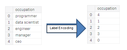![](https://raw.githubusercontent.com/WillKoehrsen/Machine-Learning-Projects/master/label_encoding.png)\n\nThis approach assumes an ordering of the categories: \"Never\" (0) < \"Rarely\" (1) < \"Most days\" (2) < \"Every day\" (3).\n\nThis assumption makes sense in this example, because there is an indisputable ranking to the categories. Not all categorical variables have a clear ordering in the values, but we refer to those that do as ordinal variables. For tree-based models (like decision trees and random forests), you can expect label encoding to work well with ordinal variables.\n","execution_count":null},{"metadata":{},"cell_type":"markdown","source":"### Points of the compass\nCompass points\n\nThe names of the compass point directions follow these rules:\n> #### 16-wind compass rose\n   - The eight half-winds are the direction points obtained by bisecting the angles between the principal winds. The half-winds are north-northeast (NNE), east-northeast (ENE), east-southeast (ESE), south-southeast (SSE), south-southwest (SSW), west-southwest (WSW), west-northwest (WNW) and north-northwest (NNW). The name of each half-wind is constructed by combining the names of the principal winds to either side, with the cardinal wind coming first and the intercardinal wind second.\n   - The eight principal winds and the eight half-winds together form the 16-wind compass rose, with each compass point at a ​22 1⁄2° angle from its two neighbours.","execution_count":null},{"metadata":{"trusted":true,"_kg_hide-input":true},"cell_type":"code","source":"# Convert wind direction into categorical feature. We can split 360 degrees into 16-wind compass rose. \n# See this: https://en.wikipedia.org/wiki/Points_of_the_compass#16-wind_compass_rose\ndef degToCompass(num):\n    val=int((num/22.5))\n    arr=[i for i in range(0,16)]\n    return arr[(val % 16)]","execution_count":null,"outputs":[]},{"metadata":{"trusted":true,"_kg_hide-input":true},"cell_type":"code","source":"le = LabelEncoder()\n\ntrain_df['primary_use'] = le.fit_transform(train_df['primary_use']).astype(np.int8)\n\ntest_df['primary_use'] = le.fit_transform(test_df['primary_use']).astype(np.int8)","execution_count":null,"outputs":[]},{"metadata":{"trusted":true,"_kg_hide-input":true},"cell_type":"code","source":"train_df['age'] = train_df['year_built'].max() - train_df['year_built'] + 1\ntest_df['age'] = test_df['year_built'].max() - test_df['year_built'] + 1","execution_count":null,"outputs":[]},{"metadata":{},"cell_type":"markdown","source":"See this, [simple FE](https://www.kaggle.com/isaienkov/lightgbm-fe-1-19): ","execution_count":null},{"metadata":{},"cell_type":"markdown","source":"# Feature Selection\n     \n#### Find the optimal feature subset using an evaluation measure. The choice of evaluation metric distinguish the three main strategies of feature selection algorithms: the wrapper strategy, the filter strategy, and the embedded strategy.\n\n    Filter methods:\n        information gain\n        chi-square test\n        correlation coefficient\n        variance threshold\n    Wrapper methods:\n        recursive feature elimination\n        sequential feature selection algorithms\n    Embedded methods:\n        L1 (LASSO) regularization\n        decision tree\n        \nIn our case, we remove some useless, redundant variables. ","execution_count":null},{"metadata":{"trusted":true,"_kg_hide-input":true},"cell_type":"code","source":"def average_imputation(df, column_name):\n    imputation = df.groupby(['timestamp'])[column_name].mean()\n    \n    df.loc[df[column_name].isnull(), column_name] = df[df[column_name].isnull()][[column_name]].apply(lambda x: imputation[df['timestamp'][x.index]].values)\n    del imputation\n    return df","execution_count":null,"outputs":[]},{"metadata":{"trusted":true,"_kg_hide-input":true},"cell_type":"code","source":"train_df = average_imputation(train_df, 'wind_speed')\ntrain_df = average_imputation(train_df, 'wind_direction')\n\nbeaufort = [(0, 0, 0.3), (1, 0.3, 1.6), (2, 1.6, 3.4), (3, 3.4, 5.5), (4, 5.5, 8), (5, 8, 10.8), (6, 10.8, 13.9), \n          (7, 13.9, 17.2), (8, 17.2, 20.8), (9, 20.8, 24.5), (10, 24.5, 28.5), (11, 28.5, 33), (12, 33, 200)]\n\nfor item in beaufort:\n    train_df.loc[(train_df['wind_speed']>=item[1]) & (train_df['wind_speed']<item[2]), 'beaufort_scale'] = item[0]\n\ntrain_df['wind_direction'] = train_df['wind_direction'].apply(degToCompass)\ntrain_df['beaufort_scale'] = train_df['beaufort_scale'].astype(np.uint8)\ntrain_df[\"wind_direction\"] = train_df['wind_direction'].astype(np.uint8)\ntrain_df[\"meter\"] = train_df['meter'].astype(np.uint8)\ntrain_df[\"site_id\"] = train_df['site_id'].astype(np.uint8)\n    \n    \ntest_df = average_imputation(test_df, 'wind_speed')\ntest_df = average_imputation(test_df, 'wind_direction')\n\nfor item in beaufort:\n    test_df.loc[(test_df['wind_speed']>=item[1]) & (test_df['wind_speed']<item[2]), 'beaufort_scale'] = item[0]\n\ntest_df['wind_direction'] = test_df['wind_direction'].apply(degToCompass)\ntest_df['wind_direction'] = test_df['wind_direction'].apply(degToCompass)\ntest_df['beaufort_scale'] = test_df['beaufort_scale'].astype(np.uint8)\ntest_df[\"wind_direction\"] = test_df['wind_direction'].astype(np.uint8)\ntest_df[\"meter\"] = test_df['meter'].astype(np.uint8)\ntest_df[\"site_id\"] = test_df['site_id'].astype(np.uint8)","execution_count":null,"outputs":[]},{"metadata":{},"cell_type":"markdown","source":"# <a id='5'>5. Feature Engineering</a>\n<a href='#1'>Top</a>","execution_count":null},{"metadata":{},"cell_type":"markdown","source":"## Datetime Features","execution_count":null},{"metadata":{"trusted":true,"_kg_hide-input":true},"cell_type":"code","source":"train_df['month_datetime'] = train_df['timestamp'].dt.month.astype(np.int8)\ntrain_df['weekofyear_datetime'] = train_df['timestamp'].dt.weekofyear.astype(np.int8)\ntrain_df['dayofyear_datetime'] = train_df['timestamp'].dt.dayofyear.astype(np.int16)\n    \ntrain_df['hour_datetime'] = train_df['timestamp'].dt.hour.astype(np.int8)  \ntrain_df['day_week'] = train_df['timestamp'].dt.dayofweek.astype(np.int8)\ntrain_df['day_month_datetime'] = train_df['timestamp'].dt.day.astype(np.int8)\ntrain_df['week_month_datetime'] = train_df['timestamp'].dt.day/7\ntrain_df['week_month_datetime'] = train_df['week_month_datetime'].apply(lambda x: math.ceil(x)).astype(np.int8)\n    \n    \ntest_df['month_datetime'] = test_df['timestamp'].dt.month.astype(np.int8)\ntest_df['weekofyear_datetime'] = test_df['timestamp'].dt.weekofyear.astype(np.int8)\ntest_df['dayofyear_datetime'] = test_df['timestamp'].dt.dayofyear.astype(np.int16)\n    \ntest_df['hour_datetime'] = test_df['timestamp'].dt.hour.astype(np.int8)\ntest_df['day_week'] = test_df['timestamp'].dt.dayofweek.astype(np.int8)\ntest_df['day_month_datetime'] = test_df['timestamp'].dt.day.astype(np.int8)\ntest_df['week_month_datetime'] = test_df['timestamp'].dt.day/7\ntest_df['week_month_datetime'] = test_df['week_month_datetime'].apply(lambda x: math.ceil(x)).astype(np.int8)\n    ","execution_count":null,"outputs":[]},{"metadata":{},"cell_type":"markdown","source":"> #### train_df data","execution_count":null},{"metadata":{"trusted":true,"_kg_hide-input":true},"cell_type":"code","source":"train_df.head()","execution_count":null,"outputs":[]},{"metadata":{},"cell_type":"markdown","source":"train_df.columns.values","execution_count":null},{"metadata":{"trusted":true,"_kg_hide-input":true},"cell_type":"code","source":"train_df.columns.values","execution_count":null,"outputs":[]},{"metadata":{"_uuid":"d629ff2d2480ee46fbb7e2d37f6b5fab8052498a","collapsed":true,"_cell_guid":"79c7e3d0-c299-4dcb-8224-4455121ee9b0","trusted":false},"cell_type":"markdown","source":"# <a id='6'>6. Exploratory Data Analysis</a>\n<a href='#1'>Top</a>\n\nExploratory Data Analysis (EDA) is an open-ended process where we calculate statistics and make figures to find trends, anomalies, patterns, or relationships within the data. ","execution_count":null},{"metadata":{},"cell_type":"markdown","source":"# <a id='6-1'>6.1 Examine the Distribution of the Target Column</a>\n<a href='#1'>Top</a>\n\n\nThe target is meter_reading - Energy consumption in kWh (or equivalent). Note that this is real data with measurement error, which we expect will impose a baseline level of modeling error.","execution_count":null},{"metadata":{"trusted":true,"_kg_hide-input":true},"cell_type":"code","source":"plt.figure(figsize = (15,5))\ntrain_df['meter_reading'].plot()","execution_count":null,"outputs":[]},{"metadata":{"trusted":true,"_kg_hide-input":true},"cell_type":"code","source":"train_df['meter_reading'].plot(kind='hist',\n                            bins=25,\n                            figsize=(15, 5),\n                           title='Distribution of Target Variable (meter_reading)')\nplt.show()","execution_count":null,"outputs":[]},{"metadata":{},"cell_type":"markdown","source":"> ### Target's log-log histogram:","execution_count":null},{"metadata":{"trusted":true,"_kg_hide-input":true},"cell_type":"code","source":"ax = np.log1p(train_df['meter_reading']).hist()\nax.set_yscale('log')\ntrain_df.meter_reading.describe()","execution_count":null,"outputs":[]},{"metadata":{},"cell_type":"markdown","source":"# <a id='6-2'>6.2 Examine Missing Values</a>\n<a href='#1'>Top</a>\n\n\nNext we can look at the number and percentage of missing values in each column. ","execution_count":null},{"metadata":{"trusted":true,"_kg_hide-input":true},"cell_type":"code","source":"# checking missing data\ntotal = train_df.isnull().sum().sort_values(ascending = False)\npercent = (train_df.isnull().sum()/train_df.isnull().count()*100).sort_values(ascending = False)\nmissing__train_data  = pd.concat([total, percent], axis=1, keys=['Total', 'Percent'])\nmissing__train_data.head(10)","execution_count":null,"outputs":[]},{"metadata":{},"cell_type":"markdown","source":"## Column Types\n\nLet's look at the number of columns of each data type. `int64` and `float64` are numeric variables ([which can be either discrete or continuous](https://stats.stackexchange.com/questions/206/what-is-the-difference-between-discrete-data-and-continuous-data)). `object` columns contain strings and are  [categorical features.](http://support.minitab.com/en-us/minitab-express/1/help-and-how-to/modeling-statistics/regression/supporting-topics/basics/what-are-categorical-discrete-and-continuous-variables/) . ","execution_count":null},{"metadata":{"trusted":true,"_kg_hide-input":true},"cell_type":"code","source":"# Number of each type of column\ntrain_df.dtypes.value_counts()","execution_count":null,"outputs":[]},{"metadata":{"trusted":true,"_kg_hide-input":true},"cell_type":"code","source":"# Number of unique classes in each object column\ntrain_df.select_dtypes('object').apply(pd.Series.nunique, axis = 0)","execution_count":null,"outputs":[]},{"metadata":{},"cell_type":"markdown","source":"# <a id='7'>7. Handling missing values</a>\n<a href='#1'>Top</a>","execution_count":null},{"metadata":{},"cell_type":"markdown","source":"Package called missingno (https://github.com/ResidentMario/missingno)\n\n     !pip install quilt","execution_count":null},{"metadata":{"trusted":true,"_kg_hide-input":true},"cell_type":"code","source":"import missingno as msno","execution_count":null,"outputs":[]},{"metadata":{},"cell_type":"markdown","source":"**Nullity Matrix**\n\nThe msno.matrix nullity matrix is a data-dense display which lets you quickly visually analyse data completion. \n","execution_count":null},{"metadata":{"trusted":true,"_kg_hide-input":true},"cell_type":"code","source":"msno.matrix(train_df.head(20000))","execution_count":null,"outputs":[]},{"metadata":{},"cell_type":"markdown","source":"**Heatmap**\n\nThe missingno correlation heatmap measures nullity correlation: how strongly the presence or absence of one variable affects the presence of another:","execution_count":null},{"metadata":{"trusted":true,"_kg_hide-input":true},"cell_type":"code","source":"a = msno.heatmap(train_df, sort='ascending')","execution_count":null,"outputs":[]},{"metadata":{},"cell_type":"markdown","source":"Manually dealing with missing values will often improve model performance. \n\nOur approach we input fillNaN = -999 just for the 4 features with most missing values.\n","execution_count":null},{"metadata":{"trusted":true,"_kg_hide-input":true},"cell_type":"code","source":"train_df['floor_count'] = train_df['floor_count'].fillna(-999).astype(np.int16)\ntest_df['floor_count'] = test_df['floor_count'].fillna(-999).astype(np.int16)\n\ntrain_df['year_built'] = train_df['year_built'].fillna(-999).astype(np.int16)\ntest_df['year_built'] = test_df['year_built'].fillna(-999).astype(np.int16)\n\ntrain_df['age'] = train_df['age'].fillna(-999).astype(np.int16)\ntest_df['age'] = test_df['age'].fillna(-999).astype(np.int16)\n\ntrain_df['cloud_coverage'] = train_df['cloud_coverage'].fillna(-999).astype(np.int16)\ntest_df['cloud_coverage'] = test_df['cloud_coverage'].fillna(-999).astype(np.int16) ","execution_count":null,"outputs":[]},{"metadata":{},"cell_type":"markdown","source":"#### Still in progress","execution_count":null},{"metadata":{},"cell_type":"markdown","source":"# <a id='8'>8.  Outlier Analysis</a>\n<a href='#1'>Top</a>","execution_count":null},{"metadata":{},"cell_type":"markdown","source":"See this: [ASHRAE: EDA and Visualization (wip)](https://www.kaggle.com/chmaxx/ashrae-eda-and-visualization-wip) (upvote this !) Not only useful but also valuable","execution_count":null},{"metadata":{"trusted":true,"_kg_hide-input":true},"cell_type":"code","source":"energy_types_dict = {0: \"electricity\", 1: \"chilledwater\", 2: \"steam\", 3: \"hotwater\"}\nenergy_types      = ['electricity', 'chilledwater', 'steam', 'hotwater']\n\nplt.figure(figsize=(16,7))\ntmp_df = train_df.meter.value_counts()\ntmp_df.index = energy_types\ntmp_df.sort_values().plot(kind=\"barh\")\nplt.title(f\"Most readings measure electricity\")\nplt.xlabel(\"Count of measurements\")\nplt.ylabel(f\"Meter type\")\nplt.tight_layout()\nplt.show()\n\nplt.figure(figsize=(16,5))\ntmp_df = train_df.groupby(\"meter\").meter_reading.sum()\ntmp_df.index = energy_types\ntmp_df.sort_values().plot(kind=\"barh\")\nplt.title(f\"Generating steam consumes most energy\")\nplt.xlabel(\"Sum of consumed energy\")\nplt.ylabel(f\"Type of energy\")\nplt.tight_layout()\nplt.show()","execution_count":null,"outputs":[]},{"metadata":{"trusted":true,"_kg_hide-input":true},"cell_type":"code","source":"plt.figure(figsize=(16,5))\nsns.distplot(train_df.meter_reading, hist=False)\nplt.title(f\"Target variable meter_reading is highly skewed\")\nplt.ylabel(\"Count of readings\")\nplt.xlabel(f\"Measured consumption\")\nplt.xlim(0, train_df.meter_reading.max() + 100_000)\nplt.tight_layout()\nplt.show()\n\nplt.figure(figsize=(16,5))\nsns.distplot(np.log1p(train_df.meter_reading))\nplt.title(f\"After log transform, meter readings look more workable but still skewed\")\nplt.ylabel(\"Count of readings\")\nplt.xlabel(f\"Measured consumption\")\nplt.xlim(0, 12)\nplt.tight_layout()\nplt.show()\n\nplt.figure(figsize=(16,5))\nfor idx in range(0,4):\n    sns.distplot(np.log1p(train_df[train_df.meter==idx].meter_reading), hist=False, label=energy_types[idx])\nplt.title(f\"After log transform, distributions of energy types look comparably skewed\")\nplt.ylabel(\"Count of readings\")\nplt.xlabel(f\"Measured consumption\")\nplt.legend()\nplt.xlim(0, 12)\nplt.tight_layout()\nplt.show()","execution_count":null,"outputs":[]},{"metadata":{"trusted":true,"_kg_hide-input":true},"cell_type":"code","source":"plt.figure(figsize=(16,7))\n_ = stats.probplot(train_df['meter_reading'], plot=plt)\nplt.title(\"Probability plot for meter_reading shows extreme skewness\")\nplt.show()","execution_count":null,"outputs":[]},{"metadata":{},"cell_type":"markdown","source":"> ### Meter readings for first 10 buildings [ 1,2,3,4,5,6,7,8,9,10]","execution_count":null},{"metadata":{"trusted":true,"_kg_hide-input":true},"cell_type":"code","source":"for bldg_id in [0, 1, 2, 2, 4,5, 6,7,8,9,10]:\n    plt.figure(figsize=(16,5))\n    tmp_df = train_df[train_df.building_id == bldg_id].copy()\n    tmp_df.set_index(\"timestamp\", inplace=True)\n    tmp_df.resample(\"D\").meter_reading.sum().plot()\n    plt.title(f\"Meter readings for building #{bldg_id} \")\n    plt.xlabel(\"Sum of readings\")\n    plt.tight_layout()\n    plt.show()","execution_count":null,"outputs":[]},{"metadata":{"trusted":true,"_kg_hide-input":true},"cell_type":"code","source":"temp_df = train_df.groupby(\"primary_use\").meter_reading.sum().sort_values()\n\nplt.figure(figsize=(16,9))\ntemp_df.plot(kind=\"barh\")\nplt.title(f\"Education buildings consume by far most of energy\")\nplt.xlabel(\"Sum of readings\")\nplt.ylabel(f\"Primary use\")\nplt.tight_layout()\nplt.show()\n\nplt.figure(figsize=(16,9))\ntemp_df[:-1].plot(kind=\"barh\")\nplt.title(f\"Among other types, office buildings consume most energy\")\nplt.xlabel(\"Sum of readings\")\nplt.ylabel(f\"Primary use w/o «Education»\")\nplt.tight_layout()\nplt.show()","execution_count":null,"outputs":[]},{"metadata":{},"cell_type":"markdown","source":"# <a id='8-1'>8.1  Outlier Distribution</a>\n<a href='#1'>Top</a>\n","execution_count":null},{"metadata":{"trusted":true,"_kg_hide-input":true},"cell_type":"code","source":"y_mean_time = train_df.groupby('timestamp').meter_reading.mean()\ny_mean_time.plot(figsize=(20, 8))","execution_count":null,"outputs":[]},{"metadata":{"trusted":true,"_kg_hide-input":true},"cell_type":"code","source":"y_mean_time.rolling(window=10).std().plot(figsize=(20, 8))\nplt.axhline(y=0.009, color='red')\nplt.axvspan(0, 905, color='green', alpha=0.1)\nplt.axvspan(906, 1505, color='red', alpha=0.1)\n","execution_count":null,"outputs":[]},{"metadata":{},"cell_type":"markdown","source":"[ASHAE Outliers: by juanmah](https://www.kaggle.com/juanmah/ashrae-outliers) (upvoted this)","execution_count":null},{"metadata":{"trusted":true,"_kg_hide-input":true},"cell_type":"code","source":"daily_train = train_df\ndaily_train['date'] = daily_train['timestamp'].dt.date\ndaily_train = daily_train.groupby(['date', 'building_id', 'meter']).sum()\ndaily_train\n\ndaily_train_agg = daily_train.groupby(['date', 'meter']).agg(['sum', 'mean', 'idxmax', 'max'])\ndaily_train_agg = daily_train_agg.reset_index()\nlevel_0 = daily_train_agg.columns.droplevel(0)\nlevel_1 = daily_train_agg.columns.droplevel(1)\nlevel_0 = ['' if x == '' else '-' + x for x in level_0]\ndaily_train_agg.columns = level_1 + level_0\ndaily_train_agg.rename_axis(None, axis=1)\ndaily_train_agg.head()","execution_count":null,"outputs":[]},{"metadata":{},"cell_type":"markdown","source":"## ⚡🔌Aggregate the data for buildings","execution_count":null},{"metadata":{"trusted":true,"_kg_hide-input":true},"cell_type":"code","source":"daily_train_agg = daily_train.groupby(['date', 'meter']).agg(['sum', 'mean', 'idxmax', 'max'])\ndaily_train_agg = daily_train_agg.reset_index()\nlevel_0 = daily_train_agg.columns.droplevel(0)\nlevel_1 = daily_train_agg.columns.droplevel(1)\nlevel_0 = ['' if x == '' else '-' + x for x in level_0]\ndaily_train_agg.columns = level_1 + level_0\ndaily_train_agg.rename_axis(None, axis=1)\ndaily_train_agg.head()","execution_count":null,"outputs":[]},{"metadata":{"trusted":true,"_kg_hide-input":true},"cell_type":"code","source":"fig_total = px.line(daily_train_agg, x='date', y='meter_reading-sum', color='meter', render_mode='svg')\nfig_total.update_layout(title='Total kWh per energy aspect')\nfig_total.show()","execution_count":null,"outputs":[]},{"metadata":{},"cell_type":"markdown","source":"The sum for each energy aspect, shows some aberrant values.","execution_count":null},{"metadata":{},"cell_type":"markdown","source":"- meter=0    **Eletricity**\n\n- meter=1    **Chilledwater**\n\n- meter=2    **Steam**\n\n- meter=3    **Hotwater**","execution_count":null},{"metadata":{"trusted":true,"_kg_hide-input":true},"cell_type":"code","source":"fig_maximum = px.line(daily_train_agg, x='date', y='meter_reading-max', color='meter', render_mode='svg')\nfig_maximum.update_layout(title='Maximum kWh value per energy aspect')\nfig_maximum.show()","execution_count":null,"outputs":[]},{"metadata":{},"cell_type":"markdown","source":"# Some 'Anomalies' - max meter reading","execution_count":null},{"metadata":{"trusted":true,"_kg_hide-input":true},"cell_type":"code","source":"daily_train_agg['building_id_max'] = [x[1] for x in daily_train_agg['meter_reading-idxmax']]\ndaily_train_agg.head()","execution_count":null,"outputs":[]},{"metadata":{},"cell_type":"markdown","source":"# <a id='10'>10. Baseline</a>\n<a href='#1'>Top</a>","execution_count":null},{"metadata":{},"cell_type":"markdown","source":"> - Drop collumns","execution_count":null},{"metadata":{"trusted":true,"_kg_hide-input":true},"cell_type":"code","source":"del train_df[\"timestamp\"], test_df[\"timestamp\"]","execution_count":null,"outputs":[]},{"metadata":{"trusted":true,"_kg_hide-input":true},"cell_type":"code","source":"categoricals = [\"site_id\", \"building_id\", \"primary_use\",  \"meter\",  \"wind_direction\"] #\"hour\", \"weekday\",","execution_count":null,"outputs":[]},{"metadata":{"trusted":true,"_kg_hide-input":true},"cell_type":"code","source":"drop_cols = [\"sea_level_pressure\", \"wind_speed\"]\n\nnumericals = [\"square_feet\", \"year_built\", \"air_temperature\", \"cloud_coverage\",\n              \"dew_temperature\", 'precip_depth_1_hr', 'floor_count', 'beaufort_scale']\n\nfeat_cols = categoricals + numericals","execution_count":null,"outputs":[]},{"metadata":{},"cell_type":"markdown","source":"> Modeling simple LGBM","execution_count":null},{"metadata":{},"cell_type":"markdown","source":"# What is K-Fold Cross Validation?","execution_count":null},{"metadata":{},"cell_type":"markdown","source":"\n**K-Fold CV[](https://medium.com/datadriveninvestor/k-fold-cross-validation-6b8518070833)** is where a given data set is split into a K number of sections/folds where each fold is used as a testing set at some point. Lets take the scenario of 5-Fold cross validation(K=5). Here, the data set is split into 5 folds. In the first iteration, the first fold is used to test the model and the rest are used to train the model. In the second iteration, 2nd fold is used as the testing set while the rest serve as the training set. This process is repeated until each fold of the 5 folds have been used as the testing set.\n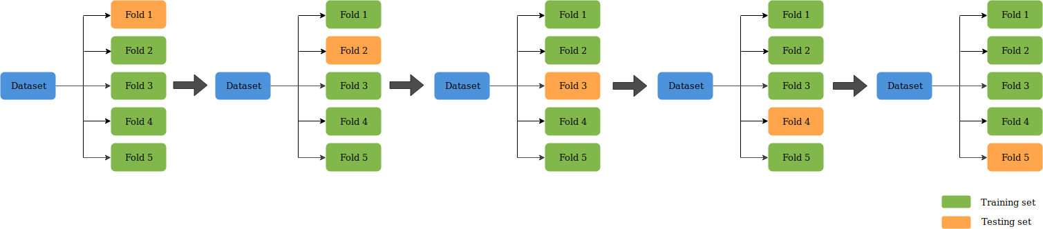![5-Fold Cross Validation](https://miro.medium.com/max/1509/1*IjKy-Zc9zVOHFzMw2GXaQw.png)","execution_count":null},{"metadata":{"trusted":true,"_kg_hide-input":true},"cell_type":"code","source":"params = {\n            'boosting_type': 'gbdt',\n            'objective': 'regression',\n            'metric': {'rmse'},\n            'subsample_freq': 1,\n            'learning_rate': 0.3,\n            'bagging_freq': 5,\n            'num_leaves': 330,\n            'feature_fraction': 0.9,\n            'lambda_l1': 1,  \n            'lambda_l2': 1\n            }\n\nfolds = 5\nseed = 666\nshuffle = False\nkf = KFold(n_splits=folds, shuffle=shuffle, random_state=seed)\n\nmodels = []\nfor train_index, val_index in kf.split(train_df[feat_cols], train_df['building_id']):\n    train_X = train_df[feat_cols].iloc[train_index]\n    val_X = train_df[feat_cols].iloc[val_index]\n    train_y = target.iloc[train_index]\n    val_y = target.iloc[val_index]\n    lgb_train = lgb.Dataset(train_X, train_y, categorical_feature=categoricals)\n    lgb_eval = lgb.Dataset(val_X, val_y, categorical_feature=categoricals)\n    gbm = lgb.train(params,\n                lgb_train,\n                num_boost_round=500,\n                valid_sets=(lgb_train, lgb_eval),\n                early_stopping_rounds=50,\n                verbose_eval = 50)\n    models.append(gbm)","execution_count":null,"outputs":[]},{"metadata":{"trusted":true,"_kg_hide-input":true},"cell_type":"code","source":"import gc\ndel train_df #, train_X, val_X, lgb_train, lgb_eval, train_y, val_y, target\ngc.collect()","execution_count":null,"outputs":[]},{"metadata":{"trusted":true,"_kg_hide-input":true},"cell_type":"code","source":"test_df = test_df[feat_cols]","execution_count":null,"outputs":[]},{"metadata":{"trusted":true,"_kg_hide-input":true},"cell_type":"code","source":"i=0\nres=[]\nstep_size = 50000\nfor j in tqdm(range(int(np.ceil(test_df.shape[0]/50000)))):\n    res.append(np.expm1(sum([model.predict(test_df.iloc[i:i+step_size]) for model in models])/folds))\n    i+=step_size","execution_count":null,"outputs":[]},{"metadata":{"trusted":true,"_kg_hide-input":true},"cell_type":"code","source":"res = np.concatenate(res)","execution_count":null,"outputs":[]}],"metadata":{"kernelspec":{"language":"python","display_name":"Python 3","name":"python3"},"language_info":{"pygments_lexer":"ipython3","nbconvert_exporter":"python","version":"3.6.4","file_extension":".py","codemirror_mode":{"name":"ipython","version":3},"name":"python","mimetype":"text/x-python"}},"nbformat":4,"nbformat_minor":4}