
First of all, thanks to Kaggle and CSIRO for organizing this competition. This is a very meaningful agricultural AI application scenario.
\nThis is my first time participating in a Kaggle CV competition, and I'm very happy and fortunate to have achieved 5th place solo (Private LB: 0.76). Throughout the competition, I conducted extensive experiments - I did about 100+ training experiments (from exp-v1 to exp-v188). Through this competition, I learned a lot about computer vision. Below is a detailed sharing of my competition solution.\n
The goal of this competition is to use pasture images to predict five key biomass components:
\n
The competition uses weighted R² score as the evaluation metric, with weighted average of R² across five targets.
\nAfter extensive ablation experiments, the following are key techniques that can stably improve scores:
\nOriginal images contain orange date timestamps, which are data noise. I used HSV color space detection and image inpainting techniques to remove these timestamps:
\ndef clean_image(img):\n \"\"\"\n Image preprocessing: Remove bottom artifacts and date stamp.\n \"\"\"\n # Detect orange date stamp in HSV space\n hsv = cv2.cvtColor(img, cv2.COLOR_RGB2HSV)\n # Define orange range\n lower = np.array([5, 150, 150])\n upper = np.array([25, 255, 255])\n mask = cv2.inRange(hsv, lower, upper)\n\n # Dilate mask to cover text edges\n mask = cv2.dilate(mask, np.ones((3, 3), np.uint8), iterations=2)\n\n # Inpaint if timestamp detected\n if np.sum(mask) > 0:\n img = cv2.inpaint(img, mask, 3, cv2.INPAINT_TELEA)\n\n return img\n
Due to the small training set size, data augmentation is crucial for preventing overfitting. I used TTA-style training strategy:
\ndef get_tta_transforms(img_size: int) -> list[A.Compose]:\n \"\"\"Returns a list of transform pipelines for TTA-style training.\"\"\"\n normalize = A.Normalize(\n mean=[0.485, 0.456, 0.406],\n std=[0.229, 0.224, 0.225]\n )\n\n # View 0: Original\n original_view = A.Compose([\n A.Resize(img_size, img_size),\n normalize,\n ToTensorV2()\n ])\n\n # View 1: Horizontal Flip\n hflip_view = A.Compose([\n A.Resize(img_size, img_size),\n A.HorizontalFlip(p=1.0),\n normalize,\n ToTensorV2()\n ])\n\n # View 2: Vertical Flip\n vflip_view = A.Compose([\n A.Resize(img_size, img_size),\n A.VerticalFlip(p=1.0),\n normalize,\n ToTensorV2()\n ])\n\n # View 3: Rotate 90 degrees\n rotate90_view = A.Compose([\n A.Resize(img_size, img_size),\n A.Rotate(limit=(90, 90), p=1.0, border_mode=0),\n normalize,\n ToTensorV2()\n ])\n\n return [hflip_view, vflip_view, rotate90_view, original_view]\nTraining Strategy:
\nIn addition to splitting the image into left and right halves (simulating stereo vision), I also added the full image as a third input stream:
\nclass BiomassDataset(Dataset):\n \"\"\"Three-stream dataset: splits 2000x1000 image into left, right, and full.\"\"\"\n\n def __getitem__(self, idx: int):\n image = self._load_image(self.image_paths[idx])\n image = clean_image(image)\n\n height, width = image.shape[:2]\n mid = width // 2\n left = image[:, :mid] # Left half\n right = image[:, mid:] # Right half\n full_image = image.copy() # Full image\n\n # Apply same transform to all three views\n left = self.transform(image=left)[\"image\"]\n right = self.transform(image=right)[\"image\"]\n full_image = self.transform(image=full_image)[\"image\"]\n\n return left, right, full_image, train_tgt, eval_tgt, species_tgt\nThis design allows the model to learn both local details (left/right views) and global context (full view) simultaneously.
\nDesign Intent: The model can automatically switch to the most suitable expert for prediction based on the specific characteristics of the input image (e.g., more green grass or more dead grass), effectively resolving feature conflicts in multi-task learning.
\nclass MetaMoE(nn.Module):\n \"\"\"Mixture-of-Experts head for main targets, outputs mean and variance.\"\"\"\n\n def __init__(self, in_dim: int, hidden: int, num_experts: int, \n out_dim: int = 1, dropout: float = 0.2):\n super().__init__()\n self.num_experts = num_experts\n\n # Gating network\n self.gate = nn.Sequential(\n nn.LayerNorm(in_dim),\n nn.Linear(in_dim, 256),\n nn.ReLU(),\n nn.Linear(256, num_experts),\n )\n\n # Expert networks (each outputs mean and variance)\n self.experts = nn.ModuleList([\n nn.Sequential(\n nn.LayerNorm(in_dim),\n nn.Linear(in_dim, hidden),\n nn.ReLU(),\n nn.Dropout(dropout),\n nn.Linear(hidden, 256),\n nn.ReLU(),\n nn.Linear(256, 2), # [mean, var_logit]\n )\n for _ in range(num_experts)\n ])\n\n def forward(self, x: torch.Tensor):\n gate_logits = self.gate(x)\n gate_weights = F.softmax(gate_logits, dim=1).unsqueeze(-1)\n expert_outs = torch.stack([expert(x) for expert in self.experts], dim=1)\n out = (expert_outs * gate_weights).sum(dim=1)\n\n pred_mean = out[:, 0:1]\n pred_var_logit = out[:, 1:2]\n pred_var = F.softplus(pred_var_logit) + 1e-6 # Ensure variance is positive\n\n return pred_mean, pred_var\n
Three Model Variants:
\nAdding extra training objectives helps the model learn richer feature representations:
\nclass BiomassModel(nn.Module):\n def __init__(self, model_name: str, pretrained: bool = True, \n pretrained_path: str = '', num_species: int = 0):\n super().__init__()\n # ... backbone initialization ...\n\n # Main regression heads (using MoE)\n self.head_total = MetaMoE(...)\n self.head_gdm = MetaMoE(...)\n self.head_green = MetaMoE(...)\n\n # Auxiliary regression heads (NDVI and Height)\n self.head_ndvi = _AuxHead(self.n_features, self.n_features // 2)\n self.head_height = _AuxHead(self.n_features, self.n_features // 2)\n\n # Optional classification heads\n if num_species > 0:\n self.head_species = self._make_classification_head(num_species)\nAuxiliary Targets:
\nDesigned loss function based on physical relationships between targets, using GaussianNLLLoss as the main loss function:
\nCore Advantages:
\nclass PhysicsConsistencyLoss(nn.Module):\n \"\"\"\n Physics consistency loss using GaussianNLLLoss\n\n Key advantages:\n - Automatic outlier handling: model learns to predict high variance for noisy samples\n - Handles heteroscedasticity: different uncertainty for different biomass levels\n - Physical constraints: Dead = Total - GDM, Clover = GDM - Green\n \"\"\"\n\n def __init__(self, weights: dict[str, float] = None):\n super().__init__()\n self.w = {\n \"total\": 0.45,\n \"gdm\": 0.2,\n \"green\": 0.1,\n \"dead\": 0.1,\n \"clover\": 0.1,\n \"ndvi\": 0.0,\n \"height\": 0.0,\n \"species\": 0.05\n }\n self.criterion = nn.GaussianNLLLoss()\n\n def forward(self, preds, targets, species_targets=None):\n # Direct prediction losses\n loss_total = self.criterion(pred_total_mean, gt_total, pred_total_var)\n loss_gdm = self.criterion(pred_gdm_mean, gt_gdm, pred_gdm_var)\n loss_green = self.criterion(pred_green_mean, gt_green, pred_green_var)\n\n # Physics constraint losses\n # Dead = Total - GDM\n pred_dead_mean = pred_total_mean - pred_gdm_mean\n pred_dead_var = pred_total_var + pred_gdm_var\n gt_dead = gt_total - gt_gdm\n loss_dead = self.criterion(pred_dead_mean, gt_dead, pred_dead_var)\n\n # Clover = GDM - Green\n pred_clover_mean = pred_gdm_mean - pred_green_mean\n pred_clover_var = pred_gdm_var + pred_green_var\n gt_clover = gt_gdm - gt_green\n loss_clover = self.criterion(pred_clover_mean, gt_clover, pred_clover_var)\n\n # Weighted total loss\n total_loss = (\n self.w[\"total\"] * loss_total +\n self.w[\"gdm\"] * loss_gdm +\n self.w[\"green\"] * loss_green +\n self.w[\"dead\"] * loss_dead +\n self.w[\"clover\"] * loss_clover\n )\n return total_loss\nSet different learning rates for pretrained Backbone and newly initialized Heads:
\nparam_groups = []\nfor name, param in model.named_parameters():\n if 'backbone' in name:\n # Backbone uses smaller lr to preserve pretrained capability\n param_groups.append({\n 'params': param, \n 'lr': cfg.finetune_lr * cfg.backbone_lr_mult # typically 0.1\n })\n elif 'head' in name:\n # Head uses larger lr for fast fitting\n param_groups.append({\n 'params': param, \n 'lr': cfg.finetune_lr * cfg.head_lr_mult # typically 1.0\n })\n else:\n param_groups.append({'params': param, 'lr': cfg.finetune_lr})\n\noptimizer = optim.AdamW(param_groups, weight_decay=cfg.weight_decay)\nRationale: Set smaller learning rate for pretrained Backbone to preserve its general feature extraction capability (prevent destroying pretrained weights), while setting larger learning rate for newly initialized Heads to quickly fit the current specific task.
\nAnalysis revealed that WA state data has different characteristics from other states:
\n# WA state special handling: Dead is 0, Total equals GDM\nif predicted_states_df is not None:\n final_pred = final_pred.merge(predicted_states_df, on='image_path', how='left')\n is_wa = final_pred['Predicted_State'] == 'WA'\n final_pred.loc[is_wa, 'Dry_Dead_g'] = 0\n final_pred.loc[is_wa, 'Dry_Total_g'] = final_pred.loc[is_wa, 'GDM_g']\nClip results based on training set target value statistics per state:
\nstate_stats = {\n 'Tas': {'Dry_Clover_g': {'min': 0.0, 'max': 71.79}, ...},\n 'NSW': {'Dry_Clover_g': {'min': 0.0, 'max': 10.10}, ...},\n 'WA': {'Dry_Clover_g': {'min': 0.0, 'max': 58.88}, ...},\n 'Vic': {'Dry_Clover_g': {'min': 0.0, 'max': 67.90}, ...}\n}\n\nfor state in state_stats.keys():\n state_mask = final_pred['Predicted_State'] == state\n for var in target_vars:\n min_val = state_stats[state][var]['min']\n max_val = state_stats[state][var]['max']\n final_pred.loc[state_mask, var] = final_pred.loc[state_mask, var].clip(\n lower=min_val, upper=max_val\n )\ndef apply_post_processing(df: pd.DataFrame) -> pd.DataFrame:\n \"\"\"Apply Clover and Dead post-processing rules.\"\"\"\n df_out = df.copy()\n if 'Dry_Clover_g' in df_out.columns:\n df_out['Dry_Clover_g'] = df_out['Dry_Clover_g'] * 0.8\n if 'Dry_Dead_g' in df_out.columns:\n mask_high = df_out['Dry_Dead_g'] > 20\n df_out.loc[mask_high, 'Dry_Dead_g'] *= 1.1\n mask_low = df_out['Dry_Dead_g'] < 10\n df_out.loc[mask_low, 'Dry_Dead_g'] *= 0.9\n return df_out\nSince the training set is quite small, the intention was to utilize all available data and simply overfit on the training set.
\n# train_df = df[df[\"fold\"] != fold].reset_index(drop=True)\n# valid_df = df[df[\"fold\"] == fold].reset_index(drop=True)\n\ntrain_df = df\nvalid_df = df\nThe final submission uses weighted ensemble of 6 models:
\n| Model | \nWeight | \nFeatures | \n
|---|---|---|
| exp-v142 | \n0.0 (State prediction only) | \nBiomassModelWithStateSpecies, extracts State info | \n
| exp-v148 | \n0.15 | \nBiomassModelWithMetaEmbedding, uses meta features | \n
| exp-v147 | \n0.20 | \nBiomassModelBasic, seed=2026 | \n
| exp-v174 | \n0.25 | \nBiomassModelBasic, random augmentation | \n
| exp-v164 | \n0.20 | \nBiomassModelBasic, TTA-style augmentation | \n
| exp-v177 | \n0.20 | \nBiomassModelBasic, adjusted loss weights | \n
Each model uses 3 TTA transforms:
\nFinal prediction is averaged.
\nImplemented dual GPU parallel inference for acceleration:
\ndef parallel_dual_gpu_inference(dataset, model_class, model_kwargs, model_states, ...):\n \"\"\"Run inference in parallel on two GPUs.\"\"\"\n # Even indices -> GPU 0, Odd indices -> GPU 1\n indices_0 = list(range(0, n, 2))\n indices_1 = list(range(1, n, 2))\n\n with ThreadPoolExecutor(max_workers=2) as executor:\n future_0 = executor.submit(inference_single_gpu, model_0, ..., device_0)\n future_1 = executor.submit(inference_single_gpu, model_1, ..., device_1)\n results_0 = future_0.result()\n results_1 = future_1.result()\n\n # Merge results\n ...\n| Hyperparameter | \nValue | \n
|---|---|
| Backbone | \nvit_large_patch16_dinov3_qkvb | \n
| Image Size | \n1024x1024 | \n
| Batch Size | \n4 | \n
| Learning Rate | \n2e-4 (finetune to 5e-5 after warm-up) | \n
| Backbone LR Multiplier | \n0.1 | \n
| Training Epochs | \n25 | \n
| MoE Experts | \n4 | \n
| MoE Hidden Dim | \n512 | \n
| Optimizer | \nAdamW | \n
| Weight Decay | \n1e-4 | \n
Based on experiment records, the following methods did not improve or were unstable:
\n| Experiment | \nDescription | \nResult | \n
|---|---|---|
| exp-v36 | \nRatio prediction | \nCV dropped from 0.58 to 0.43 | \n
| exp-v97 | \nFull image without splitting | \nCV 0.57, LB 0.52 (severe drop) | \n
| exp-v99 | \nLR 2e-4 + 20 epochs | \nCV only 0.21 | \n
| exp-v123 | \nSegmentation + attention | \nCV 0.53, LB 0.53 | \n
| exp-v168/169 | \nMamba Network | \nCV 0.80-0.89 (unstable) | \n
| exp-v180 | \nUNet original size 1000x2000 | \nLB 0.64 (significant drop) | \n
| Experiment | \nDescription | \nProblem | \n
|---|---|---|
| Huge model (exp-v170) | \nvit_huge | \nHigh CV 0.95 but LB 0.72 | \n
| 30 epochs (exp-v161) | \nIncreased epochs | \nOverfitting, Private LB dropped | \n
| Various segmentation masks | \nng/xg mask | \nPartially effective but unstable | \n
| Stage | \nExperiment | \nPublic LB | \nPrivate LB | \nKey Improvement | \n
|---|---|---|---|---|
| Baseline | \nv1 | \n0.57 | \n- | \n448 size baseline | \n
| Model Upgrade | \nv24 | \n0.65 | \n- | \nvit_large_dinov3 | \n
| Resolution | \nv32 | \n0.69 | \n- | \n512 size | \n
| Physics Loss | \nv42 | \n0.69+ | \n- | \nPhysicsConsistencyLoss | \n
| MoE | \nv44 | \n0.69 | \n- | \nMixture-of-Experts | \n
| 1024 Resolution | \nv108 | \n0.73 | \n- | \n1024 size + LR optimization | \n
| Full Training | \nv136 | \n0.74+ | \n- | \nFull dataset + Species | \n
| Seed Optimization | \nv147 | \n0.75+ | \n- | \nseed=2026 | \n
| Augmentation | \nv164 | \n0.75 | \n- | \nTTA-style augmentation | \n
| Random Aug | \nv174 | \n0.76 | \n0.65 | \nRandom augmentation selection | \n
| Ensemble | \nFinal | \n0.76 | \n0.66 | \n6-model weighted ensemble | \n
Based on submission records, the two final selected submissions:
\nSubmission selection was very difficult in this competition, mainly because:
\nI ultimately chose the submission with the highest Public LB. Although the Private LB wasn't optimal (0.66 vs 0.65 for some failed submissions), it was relatively stable.
\nI must admit there was some luck involved in this result:
\nSpecial thanks to:
\nThis solo gold medal is very important for my journey to becoming a Grandmaster! I hope this solution sharing can help everyone.
\nCode Repository: 2025-Kaggle-CSIRO-5th-solution
\nFinal Submission Notebook: CSIRO-Ensemble-Models-V12
", "messages": [ { "id": "3398385", "postDate": "01/29/2026 03:49:26", "content": "First of all, thanks to Kaggle and CSIRO for organizing this competition. This is a very meaningful agricultural AI application scenario.
\nThis is my first time participating in a Kaggle CV competition, and I'm very happy and fortunate to have achieved 5th place solo (Private LB: 0.76). Throughout the competition, I conducted extensive experiments - I did about 100+ training experiments (from exp-v1 to exp-v188). Through this competition, I learned a lot about computer vision. Below is a detailed sharing of my competition solution.\n
The goal of this competition is to use pasture images to predict five key biomass components:
\n
The competition uses weighted R² score as the evaluation metric, with weighted average of R² across five targets.
\nAfter extensive ablation experiments, the following are key techniques that can stably improve scores:
\nOriginal images contain orange date timestamps, which are data noise. I used HSV color space detection and image inpainting techniques to remove these timestamps:
\ndef clean_image(img):\n \"\"\"\n Image preprocessing: Remove bottom artifacts and date stamp.\n \"\"\"\n # Detect orange date stamp in HSV space\n hsv = cv2.cvtColor(img, cv2.COLOR_RGB2HSV)\n # Define orange range\n lower = np.array([5, 150, 150])\n upper = np.array([25, 255, 255])\n mask = cv2.inRange(hsv, lower, upper)\n\n # Dilate mask to cover text edges\n mask = cv2.dilate(mask, np.ones((3, 3), np.uint8), iterations=2)\n\n # Inpaint if timestamp detected\n if np.sum(mask) > 0:\n img = cv2.inpaint(img, mask, 3, cv2.INPAINT_TELEA)\n\n return img\n
Due to the small training set size, data augmentation is crucial for preventing overfitting. I used TTA-style training strategy:
\ndef get_tta_transforms(img_size: int) -> list[A.Compose]:\n \"\"\"Returns a list of transform pipelines for TTA-style training.\"\"\"\n normalize = A.Normalize(\n mean=[0.485, 0.456, 0.406],\n std=[0.229, 0.224, 0.225]\n )\n\n # View 0: Original\n original_view = A.Compose([\n A.Resize(img_size, img_size),\n normalize,\n ToTensorV2()\n ])\n\n # View 1: Horizontal Flip\n hflip_view = A.Compose([\n A.Resize(img_size, img_size),\n A.HorizontalFlip(p=1.0),\n normalize,\n ToTensorV2()\n ])\n\n # View 2: Vertical Flip\n vflip_view = A.Compose([\n A.Resize(img_size, img_size),\n A.VerticalFlip(p=1.0),\n normalize,\n ToTensorV2()\n ])\n\n # View 3: Rotate 90 degrees\n rotate90_view = A.Compose([\n A.Resize(img_size, img_size),\n A.Rotate(limit=(90, 90), p=1.0, border_mode=0),\n normalize,\n ToTensorV2()\n ])\n\n return [hflip_view, vflip_view, rotate90_view, original_view]\nTraining Strategy:
\nIn addition to splitting the image into left and right halves (simulating stereo vision), I also added the full image as a third input stream:
\nclass BiomassDataset(Dataset):\n \"\"\"Three-stream dataset: splits 2000x1000 image into left, right, and full.\"\"\"\n\n def __getitem__(self, idx: int):\n image = self._load_image(self.image_paths[idx])\n image = clean_image(image)\n\n height, width = image.shape[:2]\n mid = width // 2\n left = image[:, :mid] # Left half\n right = image[:, mid:] # Right half\n full_image = image.copy() # Full image\n\n # Apply same transform to all three views\n left = self.transform(image=left)[\"image\"]\n right = self.transform(image=right)[\"image\"]\n full_image = self.transform(image=full_image)[\"image\"]\n\n return left, right, full_image, train_tgt, eval_tgt, species_tgt\nThis design allows the model to learn both local details (left/right views) and global context (full view) simultaneously.
\nDesign Intent: The model can automatically switch to the most suitable expert for prediction based on the specific characteristics of the input image (e.g., more green grass or more dead grass), effectively resolving feature conflicts in multi-task learning.
\nclass MetaMoE(nn.Module):\n \"\"\"Mixture-of-Experts head for main targets, outputs mean and variance.\"\"\"\n\n def __init__(self, in_dim: int, hidden: int, num_experts: int, \n out_dim: int = 1, dropout: float = 0.2):\n super().__init__()\n self.num_experts = num_experts\n\n # Gating network\n self.gate = nn.Sequential(\n nn.LayerNorm(in_dim),\n nn.Linear(in_dim, 256),\n nn.ReLU(),\n nn.Linear(256, num_experts),\n )\n\n # Expert networks (each outputs mean and variance)\n self.experts = nn.ModuleList([\n nn.Sequential(\n nn.LayerNorm(in_dim),\n nn.Linear(in_dim, hidden),\n nn.ReLU(),\n nn.Dropout(dropout),\n nn.Linear(hidden, 256),\n nn.ReLU(),\n nn.Linear(256, 2), # [mean, var_logit]\n )\n for _ in range(num_experts)\n ])\n\n def forward(self, x: torch.Tensor):\n gate_logits = self.gate(x)\n gate_weights = F.softmax(gate_logits, dim=1).unsqueeze(-1)\n expert_outs = torch.stack([expert(x) for expert in self.experts], dim=1)\n out = (expert_outs * gate_weights).sum(dim=1)\n\n pred_mean = out[:, 0:1]\n pred_var_logit = out[:, 1:2]\n pred_var = F.softplus(pred_var_logit) + 1e-6 # Ensure variance is positive\n\n return pred_mean, pred_var\n
Three Model Variants:
\nAdding extra training objectives helps the model learn richer feature representations:
\nclass BiomassModel(nn.Module):\n def __init__(self, model_name: str, pretrained: bool = True, \n pretrained_path: str = '', num_species: int = 0):\n super().__init__()\n # ... backbone initialization ...\n\n # Main regression heads (using MoE)\n self.head_total = MetaMoE(...)\n self.head_gdm = MetaMoE(...)\n self.head_green = MetaMoE(...)\n\n # Auxiliary regression heads (NDVI and Height)\n self.head_ndvi = _AuxHead(self.n_features, self.n_features // 2)\n self.head_height = _AuxHead(self.n_features, self.n_features // 2)\n\n # Optional classification heads\n if num_species > 0:\n self.head_species = self._make_classification_head(num_species)\nAuxiliary Targets:
\nDesigned loss function based on physical relationships between targets, using GaussianNLLLoss as the main loss function:
\nCore Advantages:
\nclass PhysicsConsistencyLoss(nn.Module):\n \"\"\"\n Physics consistency loss using GaussianNLLLoss\n\n Key advantages:\n - Automatic outlier handling: model learns to predict high variance for noisy samples\n - Handles heteroscedasticity: different uncertainty for different biomass levels\n - Physical constraints: Dead = Total - GDM, Clover = GDM - Green\n \"\"\"\n\n def __init__(self, weights: dict[str, float] = None):\n super().__init__()\n self.w = {\n \"total\": 0.45,\n \"gdm\": 0.2,\n \"green\": 0.1,\n \"dead\": 0.1,\n \"clover\": 0.1,\n \"ndvi\": 0.0,\n \"height\": 0.0,\n \"species\": 0.05\n }\n self.criterion = nn.GaussianNLLLoss()\n\n def forward(self, preds, targets, species_targets=None):\n # Direct prediction losses\n loss_total = self.criterion(pred_total_mean, gt_total, pred_total_var)\n loss_gdm = self.criterion(pred_gdm_mean, gt_gdm, pred_gdm_var)\n loss_green = self.criterion(pred_green_mean, gt_green, pred_green_var)\n\n # Physics constraint losses\n # Dead = Total - GDM\n pred_dead_mean = pred_total_mean - pred_gdm_mean\n pred_dead_var = pred_total_var + pred_gdm_var\n gt_dead = gt_total - gt_gdm\n loss_dead = self.criterion(pred_dead_mean, gt_dead, pred_dead_var)\n\n # Clover = GDM - Green\n pred_clover_mean = pred_gdm_mean - pred_green_mean\n pred_clover_var = pred_gdm_var + pred_green_var\n gt_clover = gt_gdm - gt_green\n loss_clover = self.criterion(pred_clover_mean, gt_clover, pred_clover_var)\n\n # Weighted total loss\n total_loss = (\n self.w[\"total\"] * loss_total +\n self.w[\"gdm\"] * loss_gdm +\n self.w[\"green\"] * loss_green +\n self.w[\"dead\"] * loss_dead +\n self.w[\"clover\"] * loss_clover\n )\n return total_loss\nSet different learning rates for pretrained Backbone and newly initialized Heads:
\nparam_groups = []\nfor name, param in model.named_parameters():\n if 'backbone' in name:\n # Backbone uses smaller lr to preserve pretrained capability\n param_groups.append({\n 'params': param, \n 'lr': cfg.finetune_lr * cfg.backbone_lr_mult # typically 0.1\n })\n elif 'head' in name:\n # Head uses larger lr for fast fitting\n param_groups.append({\n 'params': param, \n 'lr': cfg.finetune_lr * cfg.head_lr_mult # typically 1.0\n })\n else:\n param_groups.append({'params': param, 'lr': cfg.finetune_lr})\n\noptimizer = optim.AdamW(param_groups, weight_decay=cfg.weight_decay)\nRationale: Set smaller learning rate for pretrained Backbone to preserve its general feature extraction capability (prevent destroying pretrained weights), while setting larger learning rate for newly initialized Heads to quickly fit the current specific task.
\nAnalysis revealed that WA state data has different characteristics from other states:
\n# WA state special handling: Dead is 0, Total equals GDM\nif predicted_states_df is not None:\n final_pred = final_pred.merge(predicted_states_df, on='image_path', how='left')\n is_wa = final_pred['Predicted_State'] == 'WA'\n final_pred.loc[is_wa, 'Dry_Dead_g'] = 0\n final_pred.loc[is_wa, 'Dry_Total_g'] = final_pred.loc[is_wa, 'GDM_g']\nClip results based on training set target value statistics per state:
\nstate_stats = {\n 'Tas': {'Dry_Clover_g': {'min': 0.0, 'max': 71.79}, ...},\n 'NSW': {'Dry_Clover_g': {'min': 0.0, 'max': 10.10}, ...},\n 'WA': {'Dry_Clover_g': {'min': 0.0, 'max': 58.88}, ...},\n 'Vic': {'Dry_Clover_g': {'min': 0.0, 'max': 67.90}, ...}\n}\n\nfor state in state_stats.keys():\n state_mask = final_pred['Predicted_State'] == state\n for var in target_vars:\n min_val = state_stats[state][var]['min']\n max_val = state_stats[state][var]['max']\n final_pred.loc[state_mask, var] = final_pred.loc[state_mask, var].clip(\n lower=min_val, upper=max_val\n )\ndef apply_post_processing(df: pd.DataFrame) -> pd.DataFrame:\n \"\"\"Apply Clover and Dead post-processing rules.\"\"\"\n df_out = df.copy()\n if 'Dry_Clover_g' in df_out.columns:\n df_out['Dry_Clover_g'] = df_out['Dry_Clover_g'] * 0.8\n if 'Dry_Dead_g' in df_out.columns:\n mask_high = df_out['Dry_Dead_g'] > 20\n df_out.loc[mask_high, 'Dry_Dead_g'] *= 1.1\n mask_low = df_out['Dry_Dead_g'] < 10\n df_out.loc[mask_low, 'Dry_Dead_g'] *= 0.9\n return df_out\nSince the training set is quite small, the intention was to utilize all available data and simply overfit on the training set.
\n# train_df = df[df[\"fold\"] != fold].reset_index(drop=True)\n# valid_df = df[df[\"fold\"] == fold].reset_index(drop=True)\n\ntrain_df = df\nvalid_df = df\nThe final submission uses weighted ensemble of 6 models:
\n| Model | \nWeight | \nFeatures | \n
|---|---|---|
| exp-v142 | \n0.0 (State prediction only) | \nBiomassModelWithStateSpecies, extracts State info | \n
| exp-v148 | \n0.15 | \nBiomassModelWithMetaEmbedding, uses meta features | \n
| exp-v147 | \n0.20 | \nBiomassModelBasic, seed=2026 | \n
| exp-v174 | \n0.25 | \nBiomassModelBasic, random augmentation | \n
| exp-v164 | \n0.20 | \nBiomassModelBasic, TTA-style augmentation | \n
| exp-v177 | \n0.20 | \nBiomassModelBasic, adjusted loss weights | \n
Each model uses 3 TTA transforms:
\nFinal prediction is averaged.
\nImplemented dual GPU parallel inference for acceleration:
\ndef parallel_dual_gpu_inference(dataset, model_class, model_kwargs, model_states, ...):\n \"\"\"Run inference in parallel on two GPUs.\"\"\"\n # Even indices -> GPU 0, Odd indices -> GPU 1\n indices_0 = list(range(0, n, 2))\n indices_1 = list(range(1, n, 2))\n\n with ThreadPoolExecutor(max_workers=2) as executor:\n future_0 = executor.submit(inference_single_gpu, model_0, ..., device_0)\n future_1 = executor.submit(inference_single_gpu, model_1, ..., device_1)\n results_0 = future_0.result()\n results_1 = future_1.result()\n\n # Merge results\n ...\n| Hyperparameter | \nValue | \n
|---|---|
| Backbone | \nvit_large_patch16_dinov3_qkvb | \n
| Image Size | \n1024x1024 | \n
| Batch Size | \n4 | \n
| Learning Rate | \n2e-4 (finetune to 5e-5 after warm-up) | \n
| Backbone LR Multiplier | \n0.1 | \n
| Training Epochs | \n25 | \n
| MoE Experts | \n4 | \n
| MoE Hidden Dim | \n512 | \n
| Optimizer | \nAdamW | \n
| Weight Decay | \n1e-4 | \n
Based on experiment records, the following methods did not improve or were unstable:
\n| Experiment | \nDescription | \nResult | \n
|---|---|---|
| exp-v36 | \nRatio prediction | \nCV dropped from 0.58 to 0.43 | \n
| exp-v97 | \nFull image without splitting | \nCV 0.57, LB 0.52 (severe drop) | \n
| exp-v99 | \nLR 2e-4 + 20 epochs | \nCV only 0.21 | \n
| exp-v123 | \nSegmentation + attention | \nCV 0.53, LB 0.53 | \n
| exp-v168/169 | \nMamba Network | \nCV 0.80-0.89 (unstable) | \n
| exp-v180 | \nUNet original size 1000x2000 | \nLB 0.64 (significant drop) | \n
| Experiment | \nDescription | \nProblem | \n
|---|---|---|
| Huge model (exp-v170) | \nvit_huge | \nHigh CV 0.95 but LB 0.72 | \n
| 30 epochs (exp-v161) | \nIncreased epochs | \nOverfitting, Private LB dropped | \n
| Various segmentation masks | \nng/xg mask | \nPartially effective but unstable | \n
| Stage | \nExperiment | \nPublic LB | \nPrivate LB | \nKey Improvement | \n
|---|---|---|---|---|
| Baseline | \nv1 | \n0.57 | \n- | \n448 size baseline | \n
| Model Upgrade | \nv24 | \n0.65 | \n- | \nvit_large_dinov3 | \n
| Resolution | \nv32 | \n0.69 | \n- | \n512 size | \n
| Physics Loss | \nv42 | \n0.69+ | \n- | \nPhysicsConsistencyLoss | \n
| MoE | \nv44 | \n0.69 | \n- | \nMixture-of-Experts | \n
| 1024 Resolution | \nv108 | \n0.73 | \n- | \n1024 size + LR optimization | \n
| Full Training | \nv136 | \n0.74+ | \n- | \nFull dataset + Species | \n
| Seed Optimization | \nv147 | \n0.75+ | \n- | \nseed=2026 | \n
| Augmentation | \nv164 | \n0.75 | \n- | \nTTA-style augmentation | \n
| Random Aug | \nv174 | \n0.76 | \n0.65 | \nRandom augmentation selection | \n
| Ensemble | \nFinal | \n0.76 | \n0.66 | \n6-model weighted ensemble | \n
Based on submission records, the two final selected submissions:
\nSubmission selection was very difficult in this competition, mainly because:
\nI ultimately chose the submission with the highest Public LB. Although the Private LB wasn't optimal (0.66 vs 0.65 for some failed submissions), it was relatively stable.
\nI must admit there was some luck involved in this result:
\nSpecial thanks to:
\nThis solo gold medal is very important for my journey to becoming a Grandmaster! I hope this solution sharing can help everyone.
\nCode Repository: 2025-Kaggle-CSIRO-5th-solution
\nFinal Submission Notebook: CSIRO-Ensemble-Models-V12
", "rawMarkdown": "# CSIRO Image2Biomass Prediction - 5th Place Solo Gold Medal Solution\n\nFirst of all, thanks to Kaggle and CSIRO for organizing this competition. This is a very meaningful agricultural AI application scenario.\n\n## 1. Introduction\n\nThis is my first time participating in a Kaggle CV competition, and I'm very happy and fortunate to have achieved 5th place solo (Private LB: 0.76). Throughout the competition, I conducted extensive experiments - **I did about 100+ training experiments** (from exp-v1 to exp-v188). Through this competition, I learned a lot about computer vision. Below is a detailed sharing of my competition solution.\n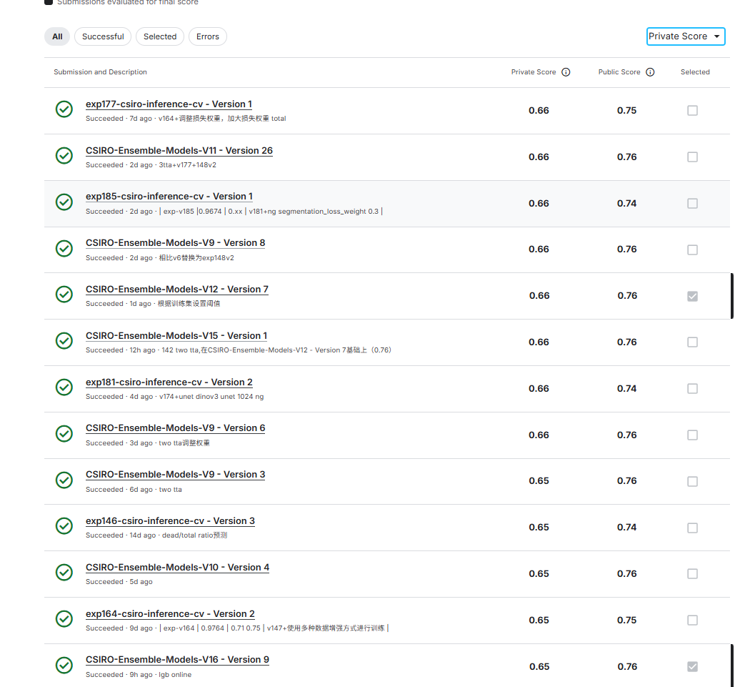\n## 2. Competition Understanding\n\n### 2.1 Problem Description\n\nThe goal of this competition is to use pasture images to predict five key biomass components:\n- **Dry_Green_g** - Dry green vegetation (excluding clover)\n- **Dry_Dead_g** - Dry dead material\n- **Dry_Clover_g** - Dry clover biomass\n- **GDM_g** - Green dry matter\n- **Dry_Total_g** - Total dry biomass\n\n### 2.2 Data Characteristics\n\n- **Small training set**: Approximately 800+ images\n- **Image size**: Original images are 2000x1000 pixels\n- **Distribution shift**: Significant differences between training and test set distributions\n- **Multi-state data**: Data from different Australian states (NSW, Tas, Vic, WA)\n- **Physical constraint relationships**: Physical relationships exist between targets\n - Dead = Total - GDM\n - Clover = GDM - Green\n\n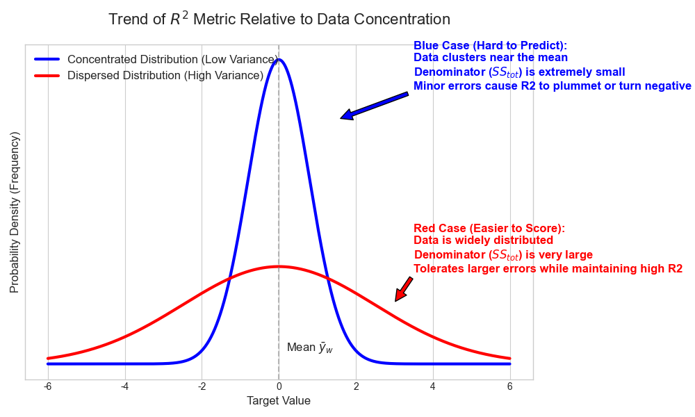\n\n### 2.3 Evaluation Metric\n\nThe competition uses weighted R² score as the evaluation metric, with weighted average of R² across five targets.\n\n## 3. Core Improvement Techniques\n\nAfter extensive ablation experiments, the following are key techniques that can stably improve scores:\n\n### 3.1 Image Preprocessing - Timestamp Removal\n\nOriginal images contain orange date timestamps, which are data noise. I used HSV color space detection and image inpainting techniques to remove these timestamps:\n\n```python\ndef clean_image(img):\n \"\"\"\n Image preprocessing: Remove bottom artifacts and date stamp.\n \"\"\"\n # Detect orange date stamp in HSV space\n hsv = cv2.cvtColor(img, cv2.COLOR_RGB2HSV)\n # Define orange range\n lower = np.array([5, 150, 150])\n upper = np.array([25, 255, 255])\n mask = cv2.inRange(hsv, lower, upper)\n\n # Dilate mask to cover text edges\n mask = cv2.dilate(mask, np.ones((3, 3), np.uint8), iterations=2)\n\n # Inpaint if timestamp detected\n if np.sum(mask) > 0:\n img = cv2.inpaint(img, mask, 3, cv2.INPAINT_TELEA)\n\n return img\n```\n\n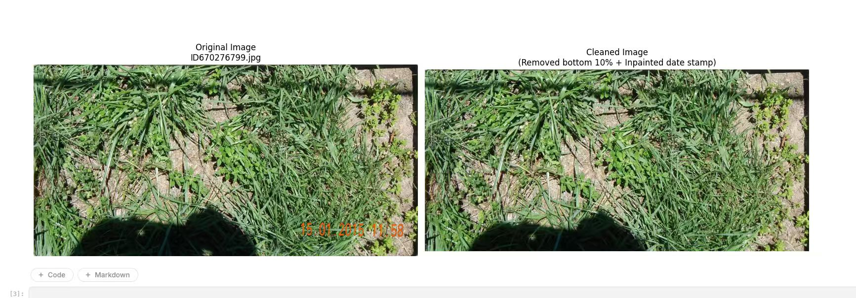\n\n### 3.2 Multiple Data Augmentations\n\nDue to the small training set size, data augmentation is crucial for preventing overfitting. I used TTA-style training strategy:\n\n```python\ndef get_tta_transforms(img_size: int) -> list[A.Compose]:\n \"\"\"Returns a list of transform pipelines for TTA-style training.\"\"\"\n normalize = A.Normalize(\n mean=[0.485, 0.456, 0.406],\n std=[0.229, 0.224, 0.225]\n )\n\n # View 0: Original\n original_view = A.Compose([\n A.Resize(img_size, img_size),\n normalize,\n ToTensorV2()\n ])\n\n # View 1: Horizontal Flip\n hflip_view = A.Compose([\n A.Resize(img_size, img_size),\n A.HorizontalFlip(p=1.0),\n normalize,\n ToTensorV2()\n ])\n\n # View 2: Vertical Flip\n vflip_view = A.Compose([\n A.Resize(img_size, img_size),\n A.VerticalFlip(p=1.0),\n normalize,\n ToTensorV2()\n ])\n\n # View 3: Rotate 90 degrees\n rotate90_view = A.Compose([\n A.Resize(img_size, img_size),\n A.Rotate(limit=(90, 90), p=1.0, border_mode=0),\n normalize,\n ToTensorV2()\n ])\n\n return [hflip_view, vflip_view, rotate90_view, original_view]\n```\n\n**Training Strategy**:\n- First 15 epochs: Train with augmented views (hflip, vflip, rotate90), equivalent to 4x data\n- Subsequent epochs: Use only original view\n- **Key finding**: Randomly selecting augmentation methods works better than sequential epoch-based selection (exp-v174)\n\n### 3.3 Multi-View Input Architecture\n\nIn addition to splitting the image into left and right halves (simulating stereo vision), I also added the full image as a third input stream:\n\n```python\nclass BiomassDataset(Dataset):\n \"\"\"Three-stream dataset: splits 2000x1000 image into left, right, and full.\"\"\"\n \n def __getitem__(self, idx: int):\n image = self._load_image(self.image_paths[idx])\n image = clean_image(image)\n\n height, width = image.shape[:2]\n mid = width // 2\n left = image[:, :mid] # Left half\n right = image[:, mid:] # Right half\n full_image = image.copy() # Full image\n\n # Apply same transform to all three views\n left = self.transform(image=left)[\"image\"]\n right = self.transform(image=right)[\"image\"]\n full_image = self.transform(image=full_image)[\"image\"]\n\n return left, right, full_image, train_tgt, eval_tgt, species_tgt\n```\n\nThis design allows the model to learn both local details (left/right views) and global context (full view) simultaneously.\n\n### 3.4 Mixture-of-Experts (MoE) Model Architecture\n\n**Design Intent**: The model can automatically switch to the most suitable expert for prediction based on the specific characteristics of the input image (e.g., more green grass or more dead grass), effectively resolving feature conflicts in multi-task learning.\n\n```python\nclass MetaMoE(nn.Module):\n \"\"\"Mixture-of-Experts head for main targets, outputs mean and variance.\"\"\"\n\n def __init__(self, in_dim: int, hidden: int, num_experts: int, \n out_dim: int = 1, dropout: float = 0.2):\n super().__init__()\n self.num_experts = num_experts\n \n # Gating network\n self.gate = nn.Sequential(\n nn.LayerNorm(in_dim),\n nn.Linear(in_dim, 256),\n nn.ReLU(),\n nn.Linear(256, num_experts),\n )\n \n # Expert networks (each outputs mean and variance)\n self.experts = nn.ModuleList([\n nn.Sequential(\n nn.LayerNorm(in_dim),\n nn.Linear(in_dim, hidden),\n nn.ReLU(),\n nn.Dropout(dropout),\n nn.Linear(hidden, 256),\n nn.ReLU(),\n nn.Linear(256, 2), # [mean, var_logit]\n )\n for _ in range(num_experts)\n ])\n\n def forward(self, x: torch.Tensor):\n gate_logits = self.gate(x)\n gate_weights = F.softmax(gate_logits, dim=1).unsqueeze(-1)\n expert_outs = torch.stack([expert(x) for expert in self.experts], dim=1)\n out = (expert_outs * gate_weights).sum(dim=1)\n\n pred_mean = out[:, 0:1]\n pred_var_logit = out[:, 1:2]\n pred_var = F.softplus(pred_var_logit) + 1e-6 # Ensure variance is positive\n\n return pred_mean, pred_var\n```\n\n\n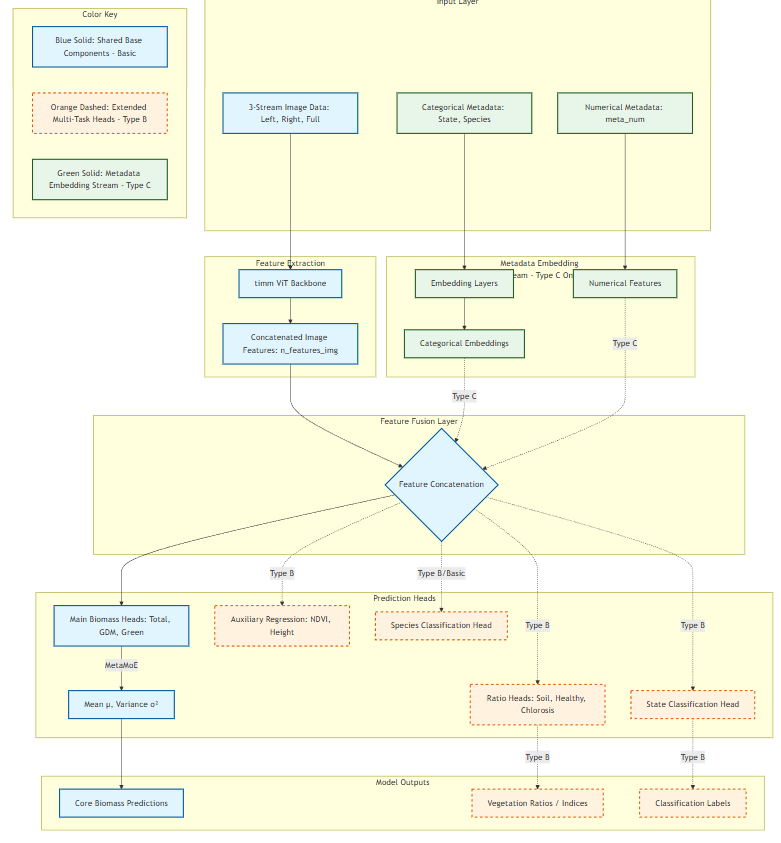\n\n**Three Model Variants**:\n- **Model Type A (BiomassModelBasic)**: Basic three-stream model (exp-v147, exp-v164, exp-v174)\n- **Model Type B (BiomassModelWithStateSpecies)**: With State/Species classification heads (exp-v142)\n- **Model Type C (BiomassModelWithMetaEmbedding)**: With meta feature embeddings (exp-v148)\n\n### 3.5 Auxiliary Training Heads\n\nAdding extra training objectives helps the model learn richer feature representations:\n\n```python\nclass BiomassModel(nn.Module):\n def __init__(self, model_name: str, pretrained: bool = True, \n pretrained_path: str = '', num_species: int = 0):\n super().__init__()\n # ... backbone initialization ...\n \n # Main regression heads (using MoE)\n self.head_total = MetaMoE(...)\n self.head_gdm = MetaMoE(...)\n self.head_green = MetaMoE(...)\n \n # Auxiliary regression heads (NDVI and Height)\n self.head_ndvi = _AuxHead(self.n_features, self.n_features // 2)\n self.head_height = _AuxHead(self.n_features, self.n_features // 2)\n \n # Optional classification heads\n if num_species > 0:\n self.head_species = self._make_classification_head(num_species)\n```\n\n**Auxiliary Targets**:\n- Pre_GSHH_NDVI (Normalized Difference Vegetation Index)\n- Height_Ave_cm (Average pasture height)\n- Species (Species classification, 15 classes)\n- State (State classification, 4 classes)\n\n### 3.6 Physics Consistency Loss\n\nDesigned loss function based on physical relationships between targets, using GaussianNLLLoss as the main loss function:\n\n**Core Advantages**:\n- Addresses the R² metric's **sensitivity to outlier errors**\n- Automatically downweights high-noise samples via GaussianNLL (avoids being biased by dirty data)\n- Uses physical constraints to ensure prediction reasonableness (avoids logical contradictions leading to large errors)\n\n```python\nclass PhysicsConsistencyLoss(nn.Module):\n \"\"\"\n Physics consistency loss using GaussianNLLLoss\n \n Key advantages:\n - Automatic outlier handling: model learns to predict high variance for noisy samples\n - Handles heteroscedasticity: different uncertainty for different biomass levels\n - Physical constraints: Dead = Total - GDM, Clover = GDM - Green\n \"\"\"\n\n def __init__(self, weights: dict[str, float] = None):\n super().__init__()\n self.w = {\n \"total\": 0.45,\n \"gdm\": 0.2,\n \"green\": 0.1,\n \"dead\": 0.1,\n \"clover\": 0.1,\n \"ndvi\": 0.0,\n \"height\": 0.0,\n \"species\": 0.05\n }\n self.criterion = nn.GaussianNLLLoss()\n\n def forward(self, preds, targets, species_targets=None):\n # Direct prediction losses\n loss_total = self.criterion(pred_total_mean, gt_total, pred_total_var)\n loss_gdm = self.criterion(pred_gdm_mean, gt_gdm, pred_gdm_var)\n loss_green = self.criterion(pred_green_mean, gt_green, pred_green_var)\n \n # Physics constraint losses\n # Dead = Total - GDM\n pred_dead_mean = pred_total_mean - pred_gdm_mean\n pred_dead_var = pred_total_var + pred_gdm_var\n gt_dead = gt_total - gt_gdm\n loss_dead = self.criterion(pred_dead_mean, gt_dead, pred_dead_var)\n \n # Clover = GDM - Green\n pred_clover_mean = pred_gdm_mean - pred_green_mean\n pred_clover_var = pred_gdm_var + pred_green_var\n gt_clover = gt_gdm - gt_green\n loss_clover = self.criterion(pred_clover_mean, gt_clover, pred_clover_var)\n \n # Weighted total loss\n total_loss = (\n self.w[\"total\"] * loss_total +\n self.w[\"gdm\"] * loss_gdm +\n self.w[\"green\"] * loss_green +\n self.w[\"dead\"] * loss_dead +\n self.w[\"clover\"] * loss_clover\n )\n return total_loss\n```\n\n### 3.7 Layer-wise Learning Rate\n\nSet different learning rates for pretrained Backbone and newly initialized Heads:\n\n```python\nparam_groups = []\nfor name, param in model.named_parameters():\n if 'backbone' in name:\n # Backbone uses smaller lr to preserve pretrained capability\n param_groups.append({\n 'params': param, \n 'lr': cfg.finetune_lr * cfg.backbone_lr_mult # typically 0.1\n })\n elif 'head' in name:\n # Head uses larger lr for fast fitting\n param_groups.append({\n 'params': param, \n 'lr': cfg.finetune_lr * cfg.head_lr_mult # typically 1.0\n })\n else:\n param_groups.append({'params': param, 'lr': cfg.finetune_lr})\n\noptimizer = optim.AdamW(param_groups, weight_decay=cfg.weight_decay)\n```\n\n**Rationale**: Set smaller learning rate for pretrained Backbone to preserve its general feature extraction capability (prevent destroying pretrained weights), while setting larger learning rate for newly initialized Heads to quickly fit the current specific task.\n\n### 3.8 Post-processing Strategies\n\n#### 3.8.1 State-based Post-processing\n\nAnalysis revealed that WA state data has different characteristics from other states:\n\n```python\n# WA state special handling: Dead is 0, Total equals GDM\nif predicted_states_df is not None:\n final_pred = final_pred.merge(predicted_states_df, on='image_path', how='left')\n is_wa = final_pred['Predicted_State'] == 'WA'\n final_pred.loc[is_wa, 'Dry_Dead_g'] = 0\n final_pred.loc[is_wa, 'Dry_Total_g'] = final_pred.loc[is_wa, 'GDM_g']\n```\n\n#### 3.8.2 Statistics-based Range Clipping\n\nClip results based on training set target value statistics per state:\n\n```python\nstate_stats = {\n 'Tas': {'Dry_Clover_g': {'min': 0.0, 'max': 71.79}, ...},\n 'NSW': {'Dry_Clover_g': {'min': 0.0, 'max': 10.10}, ...},\n 'WA': {'Dry_Clover_g': {'min': 0.0, 'max': 58.88}, ...},\n 'Vic': {'Dry_Clover_g': {'min': 0.0, 'max': 67.90}, ...}\n}\n\nfor state in state_stats.keys():\n state_mask = final_pred['Predicted_State'] == state\n for var in target_vars:\n min_val = state_stats[state][var]['min']\n max_val = state_stats[state][var]['max']\n final_pred.loc[state_mask, var] = final_pred.loc[state_mask, var].clip(\n lower=min_val, upper=max_val\n )\n```\n\n#### 3.8.3 Scaling Post-processing\n\n```python\ndef apply_post_processing(df: pd.DataFrame) -> pd.DataFrame:\n \"\"\"Apply Clover and Dead post-processing rules.\"\"\"\n df_out = df.copy()\n if 'Dry_Clover_g' in df_out.columns:\n df_out['Dry_Clover_g'] = df_out['Dry_Clover_g'] * 0.8\n if 'Dry_Dead_g' in df_out.columns:\n mask_high = df_out['Dry_Dead_g'] > 20\n df_out.loc[mask_high, 'Dry_Dead_g'] *= 1.1\n mask_low = df_out['Dry_Dead_g'] < 10\n df_out.loc[mask_low, 'Dry_Dead_g'] *= 0.9\n return df_out\n```\n### 3.9 Full Dataset Training\nSince the training set is quite small, the intention was to utilize all available data and simply overfit on the training set.\n```python\n# train_df = df[df[\"fold\"] != fold].reset_index(drop=True)\n# valid_df = df[df[\"fold\"] == fold].reset_index(drop=True)\n\ntrain_df = df\nvalid_df = df\n```\n\n## 4. Model Ensemble\n\n### 4.1 Final Ensemble Scheme\n\nThe final submission uses weighted ensemble of 6 models:\n\n| Model | Weight | Features |\n|-------|--------|----------|\n| exp-v142 | 0.0 (State prediction only) | BiomassModelWithStateSpecies, extracts State info |\n| exp-v148 | 0.15 | BiomassModelWithMetaEmbedding, uses meta features |\n| exp-v147 | 0.20 | BiomassModelBasic, seed=2026 |\n| exp-v174 | 0.25 | BiomassModelBasic, random augmentation |\n| exp-v164 | 0.20 | BiomassModelBasic, TTA-style augmentation |\n| exp-v177 | 0.20 | BiomassModelBasic, adjusted loss weights |\n\n### 4.2 TTA Inference\n\nEach model uses 3 TTA transforms:\n1. Original view\n2. Horizontal flip\n3. Vertical flip\n\nFinal prediction is averaged.\n\n### 4.3 Dual GPU Parallel Inference\n\nImplemented dual GPU parallel inference for acceleration:\n\n```python\ndef parallel_dual_gpu_inference(dataset, model_class, model_kwargs, model_states, ...):\n \"\"\"Run inference in parallel on two GPUs.\"\"\"\n # Even indices -> GPU 0, Odd indices -> GPU 1\n indices_0 = list(range(0, n, 2))\n indices_1 = list(range(1, n, 2))\n \n with ThreadPoolExecutor(max_workers=2) as executor:\n future_0 = executor.submit(inference_single_gpu, model_0, ..., device_0)\n future_1 = executor.submit(inference_single_gpu, model_1, ..., device_1)\n results_0 = future_0.result()\n results_1 = future_1.result()\n \n # Merge results\n ...\n```\n\n## 5. Key Hyperparameters\n\n| Hyperparameter | Value |\n|----------------|-------|\n| Backbone | vit_large_patch16_dinov3_qkvb |\n| Image Size | 1024x1024 |\n| Batch Size | 4 |\n| Learning Rate | 2e-4 (finetune to 5e-5 after warm-up) |\n| Backbone LR Multiplier | 0.1 |\n| Training Epochs | 25 |\n| MoE Experts | 4 |\n| MoE Hidden Dim | 512 |\n| Optimizer | AdamW |\n| Weight Decay | 1e-4 |\n\n## 6. Failed Attempts\n\nBased on experiment records, the following methods did not improve or were unstable:\n\n### 6.1 Methods That Did Not Work\n\n| Experiment | Description | Result |\n|------------|-------------|--------|\n| exp-v36 | Ratio prediction | CV dropped from 0.58 to 0.43 |\n| exp-v97 | Full image without splitting | CV 0.57, LB 0.52 (severe drop)|\n| exp-v99 | LR 2e-4 + 20 epochs | CV only 0.21 |\n| exp-v123 | Segmentation + attention | CV 0.53, LB 0.53 |\n| exp-v168/169 | Mamba Network | CV 0.80-0.89 (unstable)|\n| exp-v180 | UNet original size 1000x2000 | LB 0.64 (significant drop)|\n\n### 6.2 Unstable Methods\n\n| Experiment | Description | Problem |\n|------------|-------------|---------|\n| Huge model (exp-v170) | vit_huge | High CV 0.95 but LB 0.72 |\n| 30 epochs (exp-v161) | Increased epochs | Overfitting, Private LB dropped |\n| Various segmentation masks | ng/xg mask | Partially effective but unstable |\n\n### 6.3 Lessons Learned\n\n1. **Larger models are not always better**: Huge models easily overfit on small datasets\n2. **Training epochs need control**: ~25 epochs is the optimal balance point\n3. **Complex attention mechanisms have limited benefits**: Easily overfit on small datasets\n4. **Mamba and other sequential model architectures are not suitable for this problem**\n\n## 7. Experiment Progress\n\n### 7.1 Key Milestones\n\n| Stage | Experiment | Public LB | Private LB | Key Improvement |\n|-------|------------|-----------|------------|-----------------|\n| Baseline | v1 | 0.57 | - | 448 size baseline |\n| Model Upgrade | v24 | 0.65 | - | vit_large_dinov3 |\n| Resolution | v32 | 0.69 | - | 512 size |\n| Physics Loss | v42 | 0.69+ | - | PhysicsConsistencyLoss |\n| MoE | v44 | 0.69 | - | Mixture-of-Experts |\n| 1024 Resolution | v108 | 0.73 | - | 1024 size + LR optimization |\n| Full Training | v136 | 0.74+ | - | Full dataset + Species |\n| Seed Optimization | v147 | 0.75+ | - | seed=2026 |\n| Augmentation | v164 | 0.75 | - | TTA-style augmentation |\n| Random Aug | v174 | 0.76 | 0.65 | Random augmentation selection |\n| Ensemble | Final | 0.76 | **0.66** | 6-model weighted ensemble |\n\n### 7.2 Final Private LB Score\n\nBased on submission records, the two final selected submissions:\n- Public LB: 0.76, Private LB: 0.66 (5th Place)\n\n## 8. Conclusion and Experience Sharing\n\n### 8.1 Key Success Factors\n\n1. **Extensive experiments**: Conducted 188+ experiments, fully explored the solution space\n2. **Physical constraints**: Designed loss functions using physical relationships between targets\n3. **Diverse ensemble**: Fusion of models with different seeds, architectures, and training strategies\n4. **Data augmentation**: On small datasets, proper data augmentation is crucial\n5. **Post-processing**: Post-processing strategies based on data analysis\n\n### 8.2 About Submission Selection\n\nSubmission selection was very difficult in this competition, mainly because:\n- Small dataset size, models easily overfit\n- Distribution shift between training and test sets\n- Low correlation between Public LB and Private LB\n\nI ultimately chose the submission with the highest Public LB. Although the Private LB wasn't optimal (0.66 vs 0.65 for some failed submissions), it was relatively stable.\n\n### 8.3 Luck Factor\n\nI must admit there was some luck involved in this result:\n- Saw many top players shake-up during the final standings\n- Submission selection strategy happened to avoid pitfalls\n- Multi-model ensemble improved stability\n\n### 8.4 Acknowledgments\n\nSpecial thanks to:\n- The generous sharing from the Kaggle community\n- Discussions and notebooks from fellow Kagglers\n- CSIRO organizers for providing this meaningful competition\n\nThis solo gold medal is very important for my journey to becoming a Grandmaster! I hope this solution sharing can help everyone.\n\n---\n\n**Code Repository**: [2025-Kaggle-CSIRO-5th-solution](https://github.com/yanqiangmiffy/2025-Kaggle-CSIRO-5th-solution)\n\n**Final Submission Notebook**: [CSIRO-Ensemble-Models-V12](https://www.kaggle.com/code/quincyqiang/csiro-ensemble-models-v12?scriptVersionId=294382133)", "votes": null }, { "id": "3398390", "postDate": "01/29/2026 03:58:02", "content": "Wow, you're amazing! You actually made a lot of my 'failed' ideas work. I'm digging into your code right now to learn from it👍
", "rawMarkdown": "Wow, you're amazing! You actually made a lot of my 'failed' ideas work. I'm digging into your code right now to learn from it👍", "votes": null }, { "id": "3398402", "postDate": "01/29/2026 04:38:52", "content": "Thanks for your lot!
", "rawMarkdown": "Thanks for your lot!", "votes": null }, { "id": "3398413", "postDate": "01/29/2026 05:23:59", "content": "I saw a few top solutions. the resolution is all 1024*1024 in commm.I thingk this is the key to improve
", "rawMarkdown": "I saw a few top solutions. the resolution is all 1024*1024 in commm.I thingk this is the key to improve", "votes": null }, { "id": "3398414", "postDate": "01/29/2026 05:31:42", "content": "非常棒的方案,坚持实验的精神值得学习,恭喜你。
", "rawMarkdown": "非常棒的方案,坚持实验的精神值得学习,恭喜你。", "votes": null }, { "id": "3398416", "postDate": "01/29/2026 05:36:07", "content": "Yes,the bigger resolution did work! I tried from 224,448,512,768 to 1024
", "rawMarkdown": "Yes,the bigger resolution did work! I tried from 224,448,512,768 to 1024", "votes": null }, { "id": "3398420", "postDate": "01/29/2026 05:42:51", "content": "确实做了很多实验,也有运气成分,非常感谢认可!🍁🍁
", "rawMarkdown": "确实做了很多实验,也有运气成分,非常感谢认可!🍁🍁", "votes": null }, { "id": "3398446", "postDate": "01/29/2026 06:50:25", "content": "dinov2 pretrained on 518518,dinov2 large with 518518 can get 0.72 in public. dinov3 pretrained on 512512, 768768.Normally dinov3 should be the best in 512and 768.I don't know why it perform best with 1024*1024.additionally do you use attentionpool butilt in timm?
", "rawMarkdown": "dinov2 pretrained on 518*518,dinov2 large with 518*518 can get 0.72 in public. dinov3 pretrained on 512*512, 768*768.Normally dinov3 should be the best in 512and 768.I don't know why it perform best with 1024*1024.additionally do you use attentionpool butilt in timm?", "votes": null }, { "id": "3398458", "postDate": "01/29/2026 07:09:40", "content": "This is great , very insightful. Thanks for sharing .
", "rawMarkdown": "This is great , very insightful. Thanks for sharing .", "votes": null }, { "id": "3398470", "postDate": "01/29/2026 07:34:05", "content": "Amazing approach. \nCoincidently, I also tried the same loss function, but it was too early. I did not have the rest of the things figured out till then, like the architecture itself. And it made me think that the loss function is not working for this problem, but it was just a result of unstable experiment. I should have sticked to it, or try it again when the rest was figured out.
\nMoE is also amazing idea for this problem. I tried doing a Gradient Surgery from the paper: \"Gradient Surgery for Multi Task Learning\" to make sure all tasks are learning well, but never thought like this: If they conflict, let them conflict, just split the experts. WoW.\nI thought if we are using one of the N experts, wouldn't that simply perform like Dropout (except this is not random here) training only the activated expert, but now it is clear.
\nJust one question: Did you do some sort of analysis to see how much is each expert being activated? \nActually, when I added Task and Prompt tokens, they were converging to near same representations after the training, so I had to add an orthogonality loss. I don't see any such supervision like that here.\nAlso, did you try using more experts?
\nThanks a lot for this writeup.
", "rawMarkdown": "Amazing approach. \nCoincidently, I also tried the same loss function, but it was too early. I did not have the rest of the things figured out till then, like the architecture itself. And it made me think that the loss function is not working for this problem, but it was just a result of unstable experiment. I should have sticked to it, or try it again when the rest was figured out.\n\nMoE is also amazing idea for this problem. I tried doing a Gradient Surgery from the paper: \"Gradient Surgery for Multi Task Learning\" to make sure all tasks are learning well, but never thought like this: If they conflict, let them conflict, just split the experts. WoW.\nI thought if we are using one of the N experts, wouldn't that simply perform like Dropout (except this is not random here) training only the activated expert, but now it is clear. \n\nJust one question: Did you do some sort of analysis to see how much is each expert being activated? \nActually, when I added Task and Prompt tokens, they were converging to near same representations after the training, so I had to add an orthogonality loss. I don't see any such supervision like that here.\nAlso, did you try using more experts? \n\nThanks a lot for this writeup.", "votes": null }, { "id": "3398474", "postDate": "01/29/2026 07:41:05", "content": "Thank you for your feedback.
", "rawMarkdown": "Thank you for your feedback.", "votes": null }, { "id": "3398477", "postDate": "01/29/2026 07:43:49", "content": "I loaded it this way, setting the img_size and using average pooling.
self.backbone = timm.create_model(model_name, pretrained=pretrained, num_classes=0, global_pool=\"avg\")\nThank you for your feedback.
\nI have another question: Have you conducted any analysis to understand the activation level of each expert?\nI haven't done a specific analysis on that; I used a relatively simple configuration.
", "rawMarkdown": "Thank you for your feedback.\n```\nI have another question: Have you conducted any analysis to understand the activation level of each expert?\n```\nI haven't done a specific analysis on that; I used a relatively simple configuration.", "votes": null }, { "id": "3398544", "postDate": "01/29/2026 09:50:29", "content": "appreciate your replyly. from you not only I learned detailed code but also I learned the spirit of perseverance. you did so many experiments.It is really a big job
", "rawMarkdown": "appreciate your replyly. from you not only I learned detailed code but also I learned the spirit of perseverance. you did so many experiments.It is really a big job", "votes": null }, { "id": "3398587", "postDate": "01/29/2026 10:58:15", "content": "absolute cinema
", "rawMarkdown": "absolute cinema", "votes": null }, { "id": "3458853", "postDate": "05/16/2026 19:19:06", "content": "I added a new dataset for Image Inpainting
\nUrban Street View Image Inpainting-Random Masks
", "rawMarkdown": "I added a new dataset for Image Inpainting\n\n[Urban Street View Image Inpainting-Random Masks](https://www.kaggle.com/datasets/kannanwisen/urban-street-view-image-inpainting-random-masks)", "votes": null } ], "comments": [ { "id": 3398390, "author_name": "cudacoding", "author_url": "", "post_date": "01/29/2026 03:58:02", "content": "Wow, you're amazing! You actually made a lot of my 'failed' ideas work. I'm digging into your code right now to learn from it👍
", "votes": null, "replies": [ { "id": 3398402, "author_name": "quincyqiang", "author_url": "", "post_date": "01/29/2026 04:38:52", "content": "Thanks for your lot!
", "votes": null, "replies": [] } ] }, { "id": 3398413, "author_name": "", "author_url": "", "post_date": "01/29/2026 05:23:59", "content": "I saw a few top solutions. the resolution is all 1024*1024 in commm.I thingk this is the key to improve
", "votes": null, "replies": [ { "id": 3398416, "author_name": "quincyqiang", "author_url": "", "post_date": "01/29/2026 05:36:07", "content": "Yes,the bigger resolution did work! I tried from 224,448,512,768 to 1024
", "votes": null, "replies": [ { "id": 3398446, "author_name": "", "author_url": "", "post_date": "01/29/2026 06:50:25", "content": "dinov2 pretrained on 518518,dinov2 large with 518518 can get 0.72 in public. dinov3 pretrained on 512512, 768768.Normally dinov3 should be the best in 512and 768.I don't know why it perform best with 1024*1024.additionally do you use attentionpool butilt in timm?
", "votes": null, "replies": [ { "id": 3398477, "author_name": "quincyqiang", "author_url": "", "post_date": "01/29/2026 07:43:49", "content": "I loaded it this way, setting the img_size and using average pooling.
self.backbone = timm.create_model(model_name, pretrained=pretrained, num_classes=0, global_pool=\"avg\")\nappreciate your replyly. from you not only I learned detailed code but also I learned the spirit of perseverance. you did so many experiments.It is really a big job
", "votes": null, "replies": [] } ] } ] } ] } ] }, { "id": 3398414, "author_name": "playwithme", "author_url": "", "post_date": "01/29/2026 05:31:42", "content": "非常棒的方案,坚持实验的精神值得学习,恭喜你。
", "votes": null, "replies": [ { "id": 3398420, "author_name": "quincyqiang", "author_url": "", "post_date": "01/29/2026 05:42:51", "content": "确实做了很多实验,也有运气成分,非常感谢认可!🍁🍁
", "votes": null, "replies": [] } ] }, { "id": 3398458, "author_name": "sharmaharshit", "author_url": "", "post_date": "01/29/2026 07:09:40", "content": "This is great , very insightful. Thanks for sharing .
", "votes": null, "replies": [ { "id": 3398474, "author_name": "quincyqiang", "author_url": "", "post_date": "01/29/2026 07:41:05", "content": "Thank you for your feedback.
", "votes": null, "replies": [] } ] }, { "id": 3398470, "author_name": "komilparmar", "author_url": "", "post_date": "01/29/2026 07:34:05", "content": "Amazing approach. \nCoincidently, I also tried the same loss function, but it was too early. I did not have the rest of the things figured out till then, like the architecture itself. And it made me think that the loss function is not working for this problem, but it was just a result of unstable experiment. I should have sticked to it, or try it again when the rest was figured out.
\nMoE is also amazing idea for this problem. I tried doing a Gradient Surgery from the paper: \"Gradient Surgery for Multi Task Learning\" to make sure all tasks are learning well, but never thought like this: If they conflict, let them conflict, just split the experts. WoW.\nI thought if we are using one of the N experts, wouldn't that simply perform like Dropout (except this is not random here) training only the activated expert, but now it is clear.
\nJust one question: Did you do some sort of analysis to see how much is each expert being activated? \nActually, when I added Task and Prompt tokens, they were converging to near same representations after the training, so I had to add an orthogonality loss. I don't see any such supervision like that here.\nAlso, did you try using more experts?
\nThanks a lot for this writeup.
", "votes": null, "replies": [ { "id": 3398479, "author_name": "quincyqiang", "author_url": "", "post_date": "01/29/2026 07:45:54", "content": "Thank you for your feedback.
\nI have another question: Have you conducted any analysis to understand the activation level of each expert?\nI haven't done a specific analysis on that; I used a relatively simple configuration.
", "votes": null, "replies": [] } ] }, { "id": 3398587, "author_name": "nikitakuznetsof", "author_url": "", "post_date": "01/29/2026 10:58:15", "content": "absolute cinema
", "votes": null, "replies": [] }, { "id": 3458853, "author_name": "kannanwisen", "author_url": "", "post_date": "05/16/2026 19:19:06", "content": "I added a new dataset for Image Inpainting
\n", "votes": null, "replies": [] } ], "raw_markdown_by_id": { "3398385": "# CSIRO Image2Biomass Prediction - 5th Place Solo Gold Medal Solution\n\nFirst of all, thanks to Kaggle and CSIRO for organizing this competition. This is a very meaningful agricultural AI application scenario.\n\n## 1. Introduction\n\nThis is my first time participating in a Kaggle CV competition, and I'm very happy and fortunate to have achieved 5th place solo (Private LB: 0.76). Throughout the competition, I conducted extensive experiments - **I did about 100+ training experiments** (from exp-v1 to exp-v188). Through this competition, I learned a lot about computer vision. Below is a detailed sharing of my competition solution.\n\n## 2. Competition Understanding\n\n### 2.1 Problem Description\n\nThe goal of this competition is to use pasture images to predict five key biomass components:\n- **Dry_Green_g** - Dry green vegetation (excluding clover)\n- **Dry_Dead_g** - Dry dead material\n- **Dry_Clover_g** - Dry clover biomass\n- **GDM_g** - Green dry matter\n- **Dry_Total_g** - Total dry biomass\n\n### 2.2 Data Characteristics\n\n- **Small training set**: Approximately 800+ images\n- **Image size**: Original images are 2000x1000 pixels\n- **Distribution shift**: Significant differences between training and test set distributions\n- **Multi-state data**: Data from different Australian states (NSW, Tas, Vic, WA)\n- **Physical constraint relationships**: Physical relationships exist between targets\n - Dead = Total - GDM\n - Clover = GDM - Green\n\n\n\n### 2.3 Evaluation Metric\n\nThe competition uses weighted R² score as the evaluation metric, with weighted average of R² across five targets.\n\n## 3. Core Improvement Techniques\n\nAfter extensive ablation experiments, the following are key techniques that can stably improve scores:\n\n### 3.1 Image Preprocessing - Timestamp Removal\n\nOriginal images contain orange date timestamps, which are data noise. I used HSV color space detection and image inpainting techniques to remove these timestamps:\n\n```python\ndef clean_image(img):\n \"\"\"\n Image preprocessing: Remove bottom artifacts and date stamp.\n \"\"\"\n # Detect orange date stamp in HSV space\n hsv = cv2.cvtColor(img, cv2.COLOR_RGB2HSV)\n # Define orange range\n lower = np.array([5, 150, 150])\n upper = np.array([25, 255, 255])\n mask = cv2.inRange(hsv, lower, upper)\n\n # Dilate mask to cover text edges\n mask = cv2.dilate(mask, np.ones((3, 3), np.uint8), iterations=2)\n\n # Inpaint if timestamp detected\n if np.sum(mask) > 0:\n img = cv2.inpaint(img, mask, 3, cv2.INPAINT_TELEA)\n\n return img\n```\n\n\n\n### 3.2 Multiple Data Augmentations\n\nDue to the small training set size, data augmentation is crucial for preventing overfitting. I used TTA-style training strategy:\n\n```python\ndef get_tta_transforms(img_size: int) -> list[A.Compose]:\n \"\"\"Returns a list of transform pipelines for TTA-style training.\"\"\"\n normalize = A.Normalize(\n mean=[0.485, 0.456, 0.406],\n std=[0.229, 0.224, 0.225]\n )\n\n # View 0: Original\n original_view = A.Compose([\n A.Resize(img_size, img_size),\n normalize,\n ToTensorV2()\n ])\n\n # View 1: Horizontal Flip\n hflip_view = A.Compose([\n A.Resize(img_size, img_size),\n A.HorizontalFlip(p=1.0),\n normalize,\n ToTensorV2()\n ])\n\n # View 2: Vertical Flip\n vflip_view = A.Compose([\n A.Resize(img_size, img_size),\n A.VerticalFlip(p=1.0),\n normalize,\n ToTensorV2()\n ])\n\n # View 3: Rotate 90 degrees\n rotate90_view = A.Compose([\n A.Resize(img_size, img_size),\n A.Rotate(limit=(90, 90), p=1.0, border_mode=0),\n normalize,\n ToTensorV2()\n ])\n\n return [hflip_view, vflip_view, rotate90_view, original_view]\n```\n\n**Training Strategy**:\n- First 15 epochs: Train with augmented views (hflip, vflip, rotate90), equivalent to 4x data\n- Subsequent epochs: Use only original view\n- **Key finding**: Randomly selecting augmentation methods works better than sequential epoch-based selection (exp-v174)\n\n### 3.3 Multi-View Input Architecture\n\nIn addition to splitting the image into left and right halves (simulating stereo vision), I also added the full image as a third input stream:\n\n```python\nclass BiomassDataset(Dataset):\n \"\"\"Three-stream dataset: splits 2000x1000 image into left, right, and full.\"\"\"\n \n def __getitem__(self, idx: int):\n image = self._load_image(self.image_paths[idx])\n image = clean_image(image)\n\n height, width = image.shape[:2]\n mid = width // 2\n left = image[:, :mid] # Left half\n right = image[:, mid:] # Right half\n full_image = image.copy() # Full image\n\n # Apply same transform to all three views\n left = self.transform(image=left)[\"image\"]\n right = self.transform(image=right)[\"image\"]\n full_image = self.transform(image=full_image)[\"image\"]\n\n return left, right, full_image, train_tgt, eval_tgt, species_tgt\n```\n\nThis design allows the model to learn both local details (left/right views) and global context (full view) simultaneously.\n\n### 3.4 Mixture-of-Experts (MoE) Model Architecture\n\n**Design Intent**: The model can automatically switch to the most suitable expert for prediction based on the specific characteristics of the input image (e.g., more green grass or more dead grass), effectively resolving feature conflicts in multi-task learning.\n\n```python\nclass MetaMoE(nn.Module):\n \"\"\"Mixture-of-Experts head for main targets, outputs mean and variance.\"\"\"\n\n def __init__(self, in_dim: int, hidden: int, num_experts: int, \n out_dim: int = 1, dropout: float = 0.2):\n super().__init__()\n self.num_experts = num_experts\n \n # Gating network\n self.gate = nn.Sequential(\n nn.LayerNorm(in_dim),\n nn.Linear(in_dim, 256),\n nn.ReLU(),\n nn.Linear(256, num_experts),\n )\n \n # Expert networks (each outputs mean and variance)\n self.experts = nn.ModuleList([\n nn.Sequential(\n nn.LayerNorm(in_dim),\n nn.Linear(in_dim, hidden),\n nn.ReLU(),\n nn.Dropout(dropout),\n nn.Linear(hidden, 256),\n nn.ReLU(),\n nn.Linear(256, 2), # [mean, var_logit]\n )\n for _ in range(num_experts)\n ])\n\n def forward(self, x: torch.Tensor):\n gate_logits = self.gate(x)\n gate_weights = F.softmax(gate_logits, dim=1).unsqueeze(-1)\n expert_outs = torch.stack([expert(x) for expert in self.experts], dim=1)\n out = (expert_outs * gate_weights).sum(dim=1)\n\n pred_mean = out[:, 0:1]\n pred_var_logit = out[:, 1:2]\n pred_var = F.softplus(pred_var_logit) + 1e-6 # Ensure variance is positive\n\n return pred_mean, pred_var\n```\n\n\n\n\n**Three Model Variants**:\n- **Model Type A (BiomassModelBasic)**: Basic three-stream model (exp-v147, exp-v164, exp-v174)\n- **Model Type B (BiomassModelWithStateSpecies)**: With State/Species classification heads (exp-v142)\n- **Model Type C (BiomassModelWithMetaEmbedding)**: With meta feature embeddings (exp-v148)\n\n### 3.5 Auxiliary Training Heads\n\nAdding extra training objectives helps the model learn richer feature representations:\n\n```python\nclass BiomassModel(nn.Module):\n def __init__(self, model_name: str, pretrained: bool = True, \n pretrained_path: str = '', num_species: int = 0):\n super().__init__()\n # ... backbone initialization ...\n \n # Main regression heads (using MoE)\n self.head_total = MetaMoE(...)\n self.head_gdm = MetaMoE(...)\n self.head_green = MetaMoE(...)\n \n # Auxiliary regression heads (NDVI and Height)\n self.head_ndvi = _AuxHead(self.n_features, self.n_features // 2)\n self.head_height = _AuxHead(self.n_features, self.n_features // 2)\n \n # Optional classification heads\n if num_species > 0:\n self.head_species = self._make_classification_head(num_species)\n```\n\n**Auxiliary Targets**:\n- Pre_GSHH_NDVI (Normalized Difference Vegetation Index)\n- Height_Ave_cm (Average pasture height)\n- Species (Species classification, 15 classes)\n- State (State classification, 4 classes)\n\n### 3.6 Physics Consistency Loss\n\nDesigned loss function based on physical relationships between targets, using GaussianNLLLoss as the main loss function:\n\n**Core Advantages**:\n- Addresses the R² metric's **sensitivity to outlier errors**\n- Automatically downweights high-noise samples via GaussianNLL (avoids being biased by dirty data)\n- Uses physical constraints to ensure prediction reasonableness (avoids logical contradictions leading to large errors)\n\n```python\nclass PhysicsConsistencyLoss(nn.Module):\n \"\"\"\n Physics consistency loss using GaussianNLLLoss\n \n Key advantages:\n - Automatic outlier handling: model learns to predict high variance for noisy samples\n - Handles heteroscedasticity: different uncertainty for different biomass levels\n - Physical constraints: Dead = Total - GDM, Clover = GDM - Green\n \"\"\"\n\n def __init__(self, weights: dict[str, float] = None):\n super().__init__()\n self.w = {\n \"total\": 0.45,\n \"gdm\": 0.2,\n \"green\": 0.1,\n \"dead\": 0.1,\n \"clover\": 0.1,\n \"ndvi\": 0.0,\n \"height\": 0.0,\n \"species\": 0.05\n }\n self.criterion = nn.GaussianNLLLoss()\n\n def forward(self, preds, targets, species_targets=None):\n # Direct prediction losses\n loss_total = self.criterion(pred_total_mean, gt_total, pred_total_var)\n loss_gdm = self.criterion(pred_gdm_mean, gt_gdm, pred_gdm_var)\n loss_green = self.criterion(pred_green_mean, gt_green, pred_green_var)\n \n # Physics constraint losses\n # Dead = Total - GDM\n pred_dead_mean = pred_total_mean - pred_gdm_mean\n pred_dead_var = pred_total_var + pred_gdm_var\n gt_dead = gt_total - gt_gdm\n loss_dead = self.criterion(pred_dead_mean, gt_dead, pred_dead_var)\n \n # Clover = GDM - Green\n pred_clover_mean = pred_gdm_mean - pred_green_mean\n pred_clover_var = pred_gdm_var + pred_green_var\n gt_clover = gt_gdm - gt_green\n loss_clover = self.criterion(pred_clover_mean, gt_clover, pred_clover_var)\n \n # Weighted total loss\n total_loss = (\n self.w[\"total\"] * loss_total +\n self.w[\"gdm\"] * loss_gdm +\n self.w[\"green\"] * loss_green +\n self.w[\"dead\"] * loss_dead +\n self.w[\"clover\"] * loss_clover\n )\n return total_loss\n```\n\n### 3.7 Layer-wise Learning Rate\n\nSet different learning rates for pretrained Backbone and newly initialized Heads:\n\n```python\nparam_groups = []\nfor name, param in model.named_parameters():\n if 'backbone' in name:\n # Backbone uses smaller lr to preserve pretrained capability\n param_groups.append({\n 'params': param, \n 'lr': cfg.finetune_lr * cfg.backbone_lr_mult # typically 0.1\n })\n elif 'head' in name:\n # Head uses larger lr for fast fitting\n param_groups.append({\n 'params': param, \n 'lr': cfg.finetune_lr * cfg.head_lr_mult # typically 1.0\n })\n else:\n param_groups.append({'params': param, 'lr': cfg.finetune_lr})\n\noptimizer = optim.AdamW(param_groups, weight_decay=cfg.weight_decay)\n```\n\n**Rationale**: Set smaller learning rate for pretrained Backbone to preserve its general feature extraction capability (prevent destroying pretrained weights), while setting larger learning rate for newly initialized Heads to quickly fit the current specific task.\n\n### 3.8 Post-processing Strategies\n\n#### 3.8.1 State-based Post-processing\n\nAnalysis revealed that WA state data has different characteristics from other states:\n\n```python\n# WA state special handling: Dead is 0, Total equals GDM\nif predicted_states_df is not None:\n final_pred = final_pred.merge(predicted_states_df, on='image_path', how='left')\n is_wa = final_pred['Predicted_State'] == 'WA'\n final_pred.loc[is_wa, 'Dry_Dead_g'] = 0\n final_pred.loc[is_wa, 'Dry_Total_g'] = final_pred.loc[is_wa, 'GDM_g']\n```\n\n#### 3.8.2 Statistics-based Range Clipping\n\nClip results based on training set target value statistics per state:\n\n```python\nstate_stats = {\n 'Tas': {'Dry_Clover_g': {'min': 0.0, 'max': 71.79}, ...},\n 'NSW': {'Dry_Clover_g': {'min': 0.0, 'max': 10.10}, ...},\n 'WA': {'Dry_Clover_g': {'min': 0.0, 'max': 58.88}, ...},\n 'Vic': {'Dry_Clover_g': {'min': 0.0, 'max': 67.90}, ...}\n}\n\nfor state in state_stats.keys():\n state_mask = final_pred['Predicted_State'] == state\n for var in target_vars:\n min_val = state_stats[state][var]['min']\n max_val = state_stats[state][var]['max']\n final_pred.loc[state_mask, var] = final_pred.loc[state_mask, var].clip(\n lower=min_val, upper=max_val\n )\n```\n\n#### 3.8.3 Scaling Post-processing\n\n```python\ndef apply_post_processing(df: pd.DataFrame) -> pd.DataFrame:\n \"\"\"Apply Clover and Dead post-processing rules.\"\"\"\n df_out = df.copy()\n if 'Dry_Clover_g' in df_out.columns:\n df_out['Dry_Clover_g'] = df_out['Dry_Clover_g'] * 0.8\n if 'Dry_Dead_g' in df_out.columns:\n mask_high = df_out['Dry_Dead_g'] > 20\n df_out.loc[mask_high, 'Dry_Dead_g'] *= 1.1\n mask_low = df_out['Dry_Dead_g'] < 10\n df_out.loc[mask_low, 'Dry_Dead_g'] *= 0.9\n return df_out\n```\n### 3.9 Full Dataset Training\nSince the training set is quite small, the intention was to utilize all available data and simply overfit on the training set.\n```python\n# train_df = df[df[\"fold\"] != fold].reset_index(drop=True)\n# valid_df = df[df[\"fold\"] == fold].reset_index(drop=True)\n\ntrain_df = df\nvalid_df = df\n```\n\n## 4. Model Ensemble\n\n### 4.1 Final Ensemble Scheme\n\nThe final submission uses weighted ensemble of 6 models:\n\n| Model | Weight | Features |\n|-------|--------|----------|\n| exp-v142 | 0.0 (State prediction only) | BiomassModelWithStateSpecies, extracts State info |\n| exp-v148 | 0.15 | BiomassModelWithMetaEmbedding, uses meta features |\n| exp-v147 | 0.20 | BiomassModelBasic, seed=2026 |\n| exp-v174 | 0.25 | BiomassModelBasic, random augmentation |\n| exp-v164 | 0.20 | BiomassModelBasic, TTA-style augmentation |\n| exp-v177 | 0.20 | BiomassModelBasic, adjusted loss weights |\n\n### 4.2 TTA Inference\n\nEach model uses 3 TTA transforms:\n1. Original view\n2. Horizontal flip\n3. Vertical flip\n\nFinal prediction is averaged.\n\n### 4.3 Dual GPU Parallel Inference\n\nImplemented dual GPU parallel inference for acceleration:\n\n```python\ndef parallel_dual_gpu_inference(dataset, model_class, model_kwargs, model_states, ...):\n \"\"\"Run inference in parallel on two GPUs.\"\"\"\n # Even indices -> GPU 0, Odd indices -> GPU 1\n indices_0 = list(range(0, n, 2))\n indices_1 = list(range(1, n, 2))\n \n with ThreadPoolExecutor(max_workers=2) as executor:\n future_0 = executor.submit(inference_single_gpu, model_0, ..., device_0)\n future_1 = executor.submit(inference_single_gpu, model_1, ..., device_1)\n results_0 = future_0.result()\n results_1 = future_1.result()\n \n # Merge results\n ...\n```\n\n## 5. Key Hyperparameters\n\n| Hyperparameter | Value |\n|----------------|-------|\n| Backbone | vit_large_patch16_dinov3_qkvb |\n| Image Size | 1024x1024 |\n| Batch Size | 4 |\n| Learning Rate | 2e-4 (finetune to 5e-5 after warm-up) |\n| Backbone LR Multiplier | 0.1 |\n| Training Epochs | 25 |\n| MoE Experts | 4 |\n| MoE Hidden Dim | 512 |\n| Optimizer | AdamW |\n| Weight Decay | 1e-4 |\n\n## 6. Failed Attempts\n\nBased on experiment records, the following methods did not improve or were unstable:\n\n### 6.1 Methods That Did Not Work\n\n| Experiment | Description | Result |\n|------------|-------------|--------|\n| exp-v36 | Ratio prediction | CV dropped from 0.58 to 0.43 |\n| exp-v97 | Full image without splitting | CV 0.57, LB 0.52 (severe drop)|\n| exp-v99 | LR 2e-4 + 20 epochs | CV only 0.21 |\n| exp-v123 | Segmentation + attention | CV 0.53, LB 0.53 |\n| exp-v168/169 | Mamba Network | CV 0.80-0.89 (unstable)|\n| exp-v180 | UNet original size 1000x2000 | LB 0.64 (significant drop)|\n\n### 6.2 Unstable Methods\n\n| Experiment | Description | Problem |\n|------------|-------------|---------|\n| Huge model (exp-v170) | vit_huge | High CV 0.95 but LB 0.72 |\n| 30 epochs (exp-v161) | Increased epochs | Overfitting, Private LB dropped |\n| Various segmentation masks | ng/xg mask | Partially effective but unstable |\n\n### 6.3 Lessons Learned\n\n1. **Larger models are not always better**: Huge models easily overfit on small datasets\n2. **Training epochs need control**: ~25 epochs is the optimal balance point\n3. **Complex attention mechanisms have limited benefits**: Easily overfit on small datasets\n4. **Mamba and other sequential model architectures are not suitable for this problem**\n\n## 7. Experiment Progress\n\n### 7.1 Key Milestones\n\n| Stage | Experiment | Public LB | Private LB | Key Improvement |\n|-------|------------|-----------|------------|-----------------|\n| Baseline | v1 | 0.57 | - | 448 size baseline |\n| Model Upgrade | v24 | 0.65 | - | vit_large_dinov3 |\n| Resolution | v32 | 0.69 | - | 512 size |\n| Physics Loss | v42 | 0.69+ | - | PhysicsConsistencyLoss |\n| MoE | v44 | 0.69 | - | Mixture-of-Experts |\n| 1024 Resolution | v108 | 0.73 | - | 1024 size + LR optimization |\n| Full Training | v136 | 0.74+ | - | Full dataset + Species |\n| Seed Optimization | v147 | 0.75+ | - | seed=2026 |\n| Augmentation | v164 | 0.75 | - | TTA-style augmentation |\n| Random Aug | v174 | 0.76 | 0.65 | Random augmentation selection |\n| Ensemble | Final | 0.76 | **0.66** | 6-model weighted ensemble |\n\n### 7.2 Final Private LB Score\n\nBased on submission records, the two final selected submissions:\n- Public LB: 0.76, Private LB: 0.66 (5th Place)\n\n## 8. Conclusion and Experience Sharing\n\n### 8.1 Key Success Factors\n\n1. **Extensive experiments**: Conducted 188+ experiments, fully explored the solution space\n2. **Physical constraints**: Designed loss functions using physical relationships between targets\n3. **Diverse ensemble**: Fusion of models with different seeds, architectures, and training strategies\n4. **Data augmentation**: On small datasets, proper data augmentation is crucial\n5. **Post-processing**: Post-processing strategies based on data analysis\n\n### 8.2 About Submission Selection\n\nSubmission selection was very difficult in this competition, mainly because:\n- Small dataset size, models easily overfit\n- Distribution shift between training and test sets\n- Low correlation between Public LB and Private LB\n\nI ultimately chose the submission with the highest Public LB. Although the Private LB wasn't optimal (0.66 vs 0.65 for some failed submissions), it was relatively stable.\n\n### 8.3 Luck Factor\n\nI must admit there was some luck involved in this result:\n- Saw many top players shake-up during the final standings\n- Submission selection strategy happened to avoid pitfalls\n- Multi-model ensemble improved stability\n\n### 8.4 Acknowledgments\n\nSpecial thanks to:\n- The generous sharing from the Kaggle community\n- Discussions and notebooks from fellow Kagglers\n- CSIRO organizers for providing this meaningful competition\n\nThis solo gold medal is very important for my journey to becoming a Grandmaster! I hope this solution sharing can help everyone.\n\n---\n\n**Code Repository**: [2025-Kaggle-CSIRO-5th-solution](https://github.com/yanqiangmiffy/2025-Kaggle-CSIRO-5th-solution)\n\n**Final Submission Notebook**: [CSIRO-Ensemble-Models-V12](https://www.kaggle.com/code/quincyqiang/csiro-ensemble-models-v12?scriptVersionId=294382133)", "3398390": "Wow, you're amazing! You actually made a lot of my 'failed' ideas work. I'm digging into your code right now to learn from it👍", "3398402": "Thanks for your lot!", "3398413": "I saw a few top solutions. the resolution is all 1024*1024 in commm.I thingk this is the key to improve", "3398414": "非常棒的方案,坚持实验的精神值得学习,恭喜你。", "3398416": "Yes,the bigger resolution did work! I tried from 224,448,512,768 to 1024", "3398420": "确实做了很多实验,也有运气成分,非常感谢认可!🍁🍁", "3398446": "dinov2 pretrained on 518*518,dinov2 large with 518*518 can get 0.72 in public. dinov3 pretrained on 512*512, 768*768.Normally dinov3 should be the best in 512and 768.I don't know why it perform best with 1024*1024.additionally do you use attentionpool butilt in timm?", "3398458": "This is great , very insightful. Thanks for sharing .", "3398470": "Amazing approach. \nCoincidently, I also tried the same loss function, but it was too early. I did not have the rest of the things figured out till then, like the architecture itself. And it made me think that the loss function is not working for this problem, but it was just a result of unstable experiment. I should have sticked to it, or try it again when the rest was figured out.\n\nMoE is also amazing idea for this problem. I tried doing a Gradient Surgery from the paper: \"Gradient Surgery for Multi Task Learning\" to make sure all tasks are learning well, but never thought like this: If they conflict, let them conflict, just split the experts. WoW.\nI thought if we are using one of the N experts, wouldn't that simply perform like Dropout (except this is not random here) training only the activated expert, but now it is clear. \n\nJust one question: Did you do some sort of analysis to see how much is each expert being activated? \nActually, when I added Task and Prompt tokens, they were converging to near same representations after the training, so I had to add an orthogonality loss. I don't see any such supervision like that here.\nAlso, did you try using more experts? \n\nThanks a lot for this writeup.", "3398474": "Thank you for your feedback.", "3398477": "I loaded it this way, setting the `img_size` and using average pooling.\n```\nself.backbone = timm.create_model(model_name, pretrained=pretrained, num_classes=0, global_pool=\"avg\")\n```", "3398479": "Thank you for your feedback.\n```\nI have another question: Have you conducted any analysis to understand the activation level of each expert?\n```\nI haven't done a specific analysis on that; I used a relatively simple configuration.", "3398544": "appreciate your replyly. from you not only I learned detailed code but also I learned the spirit of perseverance. you did so many experiments.It is really a big job", "3398587": "absolute cinema", "3458853": "I added a new dataset for Image Inpainting\n\n[Urban Street View Image Inpainting-Random Masks](https://www.kaggle.com/datasets/kannanwisen/urban-street-view-image-inpainting-random-masks)" }, "source": "meta" }