
This has been one of the most frustrating competitions I’ve participated in so far. Everything felt extremely random. I tried countless approaches, but only a handful of them actually worked (or maybe not? 😂). The CV and LB fluctuated unpredictably. In the end, I had no choice but to ensemble everything I had tried - without even knowing whether it truly helped - and hope for minimal shake-up.
\nNow that the private leaderboard has been revealed, I’ve revisited all my experiments. This finally allows me to gain more confidence in what genuinely worked and what didn’t. I will ignore the many approaches that turned out to be ineffective, and summarize only the useful findings as concisely as possible:
\nThere are mainly two variations that are eventually included in my ensembles:
\n

Type A is essentially adopted from public notebooks, where the film layer is the most effective component:
\nclass FiLM(nn.Module):\n def __init__(self, feat_dim):\n super().__init__()\n hidden = max(32, feat_dim // 2)\n self.mlp = nn.Sequential(\n nn.Linear(feat_dim, hidden),\n nn.ReLU(inplace=True),\n nn.Linear(hidden, feat_dim * 2) # output gamma + beta\n )\n def forward(self, context):\n gamma_beta = self.mlp(context)\n return torch.chunk(gamma_beta, 2, dim=1) # (gamma, beta)\nI simplified the original approach by discarding techniques such as left–right feature concatenation, which I believe is unnecessary, since there is no inherent left–right structure in the images.
\nType B, based on my experiments, consistently yields better results on CV and slightly better results on LB. It leverages the intuition that biomass weight can be estimated at the tile level and then aggregated to obtain the final prediction. Compared to Type A, which relies solely on mean-pooled features fed into the prediction heads, Type B allows the heads to capture richer local information, leading to more accurate final results.
\nIn terms of variations of heads, I tried 3 heads (green, gdm, total), 4 heads (green, clover, gdm, total), and 5 heads. 5 heads gave the worst results. 3 heads and 4 heads are pretty much identical in CV and LB, so I too included both of them in my ensembles.
\nOverall, my takeaway is that the backbone is what really drives leaderboard performance - ViT Huge > ViT Large > ViT Small. Beyond that, adding more complex structures (attention, gating, mean–max pooling, etc.) doesn’t help at all given the small image size and dataset. Keeping things simple and elegant works best.
\nThis is the most tricky part, I tried countless methods. This is the only way I found slightly impoved my CV and public LB (and private LB as well):
\n

In augmented data treatment, a sliding starting point is randomly generated during training and from where only 6 tiles are cut out (plus 2 masking tiles) as input. This approach allows the model to see more variations of the image instead of a fixed 8-tile partition. When this approach is used in model structure Type B (tile-level heads) mentioned above, the targets need to be multiplied by 6/8=0.75, because fewer tiles essentially means fewer biomass.
\nThe probabilty of using augmented tiling in dataloader is set to 0.5, of which the loss weight is set to 0.5 too.
\nThere are also some standard training settings which are not decisive on their own, but proved to be optimal based on my experience:
\nTraining are set in two stages, with an early stop patience of 12:
\nOther settings:
\nweight_decay = 0.05\ndropout = 0.3\nloss_w = [0.1, 0.1, 0.1, 0.1, 0.1] # in order of [green, dead, clover, gdm, total], I found this slightly better than [0.1, 0.1, 0.1, 0.2, 0.5] \nLoss is computed with huber_loss:
\nresid = (preds - targets) / scale # (B,5)\nw = torch.tensor(loss_w, device=preds.device, dtype=preds.dtype)\nloss_per_sample = (F.huber_loss(\n resid, torch.zeros_like(resid),\n delta=1.0,\n reduction=\"none\"\n ) * w).sum(dim=1) # (B,)\nI picked two submissions:
\nEvenually both of them achieve a private LB of 0.64. However my best submission is a single model using the techniques I summarized above, which got 0.65 in private LB. Sigh~
", "messages": [ { "id": 3398395, "postDate": "2026-01-29T04:13:58.733Z", "content": "This has been one of the most frustrating competitions I’ve participated in so far. Everything felt extremely random. I tried countless approaches, but only a handful of them actually worked (or maybe not? 😂). The CV and LB fluctuated unpredictably. In the end, I had no choice but to ensemble everything I had tried - without even knowing whether it truly helped - and hope for minimal shake-up.
\nNow that the private leaderboard has been revealed, I’ve revisited all my experiments. This finally allows me to gain more confidence in what genuinely worked and what didn’t. I will ignore the many approaches that turned out to be ineffective, and summarize only the useful findings as concisely as possible:
\nThere are mainly two variations that are eventually included in my ensembles:
\n
Type A is essentially adopted from public notebooks, where the film layer is the most effective component:
\nclass FiLM(nn.Module):\n def __init__(self, feat_dim):\n super().__init__()\n hidden = max(32, feat_dim // 2)\n self.mlp = nn.Sequential(\n nn.Linear(feat_dim, hidden),\n nn.ReLU(inplace=True),\n nn.Linear(hidden, feat_dim * 2) # output gamma + beta\n )\n def forward(self, context):\n gamma_beta = self.mlp(context)\n return torch.chunk(gamma_beta, 2, dim=1) # (gamma, beta)\nI simplified the original approach by discarding techniques such as left–right feature concatenation, which I believe is unnecessary, since there is no inherent left–right structure in the images.
\nType B, based on my experiments, consistently yields better results on CV and slightly better results on LB. It leverages the intuition that biomass weight can be estimated at the tile level and then aggregated to obtain the final prediction. Compared to Type A, which relies solely on mean-pooled features fed into the prediction heads, Type B allows the heads to capture richer local information, leading to more accurate final results.
\nIn terms of variations of heads, I tried 3 heads (green, gdm, total), 4 heads (green, clover, gdm, total), and 5 heads. 5 heads gave the worst results. 3 heads and 4 heads are pretty much identical in CV and LB, so I too included both of them in my ensembles.
\nOverall, my takeaway is that the backbone is what really drives leaderboard performance - ViT Huge > ViT Large > ViT Small. Beyond that, adding more complex structures (attention, gating, mean–max pooling, etc.) doesn’t help at all given the small image size and dataset. Keeping things simple and elegant works best.
\nThis is the most tricky part, I tried countless methods. This is the only way I found slightly impoved my CV and public LB (and private LB as well):
\n
In augmented data treatment, a sliding starting point is randomly generated during training and from where only 6 tiles are cut out (plus 2 masking tiles) as input. This approach allows the model to see more variations of the image instead of a fixed 8-tile partition. When this approach is used in model structure Type B (tile-level heads) mentioned above, the targets need to be multiplied by 6/8=0.75, because fewer tiles essentially means fewer biomass.
\nThe probabilty of using augmented tiling in dataloader is set to 0.5, of which the loss weight is set to 0.5 too.
\nThere are also some standard training settings which are not decisive on their own, but proved to be optimal based on my experience:
\nTraining are set in two stages, with an early stop patience of 12:
\nOther settings:
\nweight_decay = 0.05\ndropout = 0.3\nloss_w = [0.1, 0.1, 0.1, 0.1, 0.1] # in order of [green, dead, clover, gdm, total], I found this slightly better than [0.1, 0.1, 0.1, 0.2, 0.5] \nLoss is computed with huber_loss:
\nresid = (preds - targets) / scale # (B,5)\nw = torch.tensor(loss_w, device=preds.device, dtype=preds.dtype)\nloss_per_sample = (F.huber_loss(\n resid, torch.zeros_like(resid),\n delta=1.0,\n reduction=\"none\"\n ) * w).sum(dim=1) # (B,)\nI picked two submissions:
\nEvenually both of them achieve a private LB of 0.64. However my best submission is a single model using the techniques I summarized above, which got 0.65 in private LB. Sigh~
", "rawMarkdown": "This has been one of the most frustrating competitions I’ve participated in so far. Everything felt extremely random. I tried countless approaches, but only a handful of them actually worked (or maybe not? 😂). The CV and LB fluctuated unpredictably. In the end, I had no choice but to ensemble everything I had tried - without even knowing whether it truly helped - and hope for minimal shake-up.\n\nNow that the private leaderboard has been revealed, I’ve revisited all my experiments. This finally allows me to gain more confidence in what genuinely worked and what didn’t. I will ignore the many approaches that turned out to be ineffective, and summarize only the useful findings as concisely as possible:\n\n---\n# Model structures\n\nThere are mainly two variations that are eventually included in my ensembles:\n\n### Type A (heads take mean-pooled feature as input):\n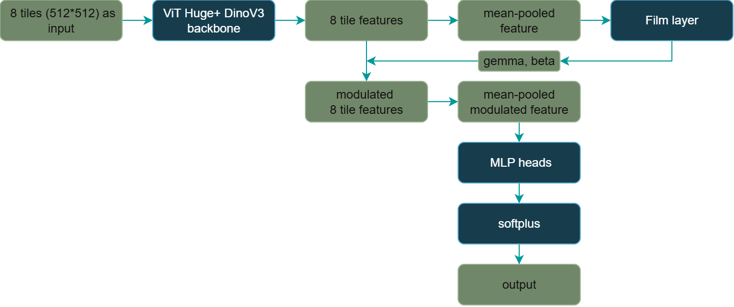\n\n### Type B (heads take tile-level features as input):\n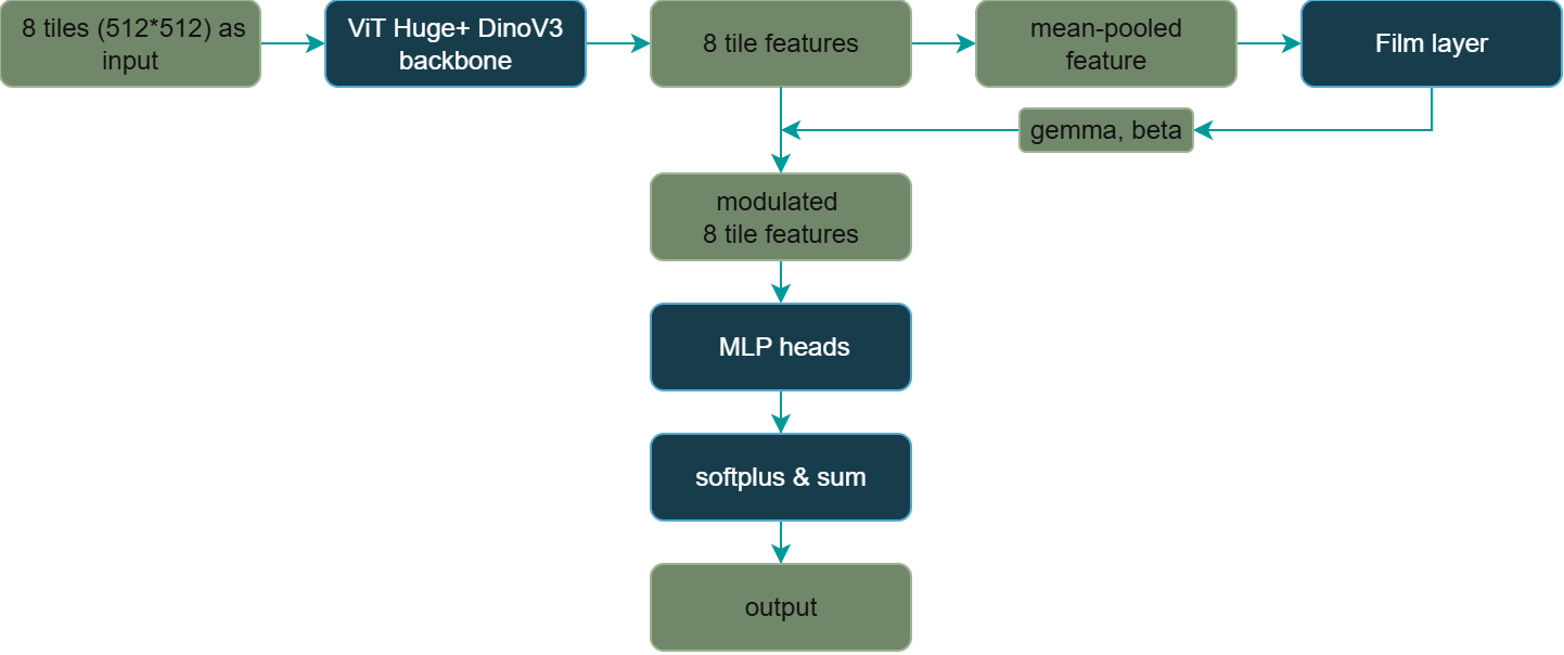\n\nType A is essentially adopted from public notebooks, where the film layer is the most effective component:\n\n class FiLM(nn.Module):\n def __init__(self, feat_dim):\n super().__init__()\n hidden = max(32, feat_dim // 2)\n self.mlp = nn.Sequential(\n nn.Linear(feat_dim, hidden),\n nn.ReLU(inplace=True),\n nn.Linear(hidden, feat_dim * 2) # output gamma + beta\n )\n def forward(self, context):\n gamma_beta = self.mlp(context)\n return torch.chunk(gamma_beta, 2, dim=1) # (gamma, beta)\n\nI simplified the original approach by discarding techniques such as left–right feature concatenation, which I believe is unnecessary, since there is no inherent left–right structure in the images.\n\nType B, based on my experiments, consistently yields better results on CV and slightly better results on LB. It leverages the intuition that biomass weight can be estimated at the tile level and then aggregated to obtain the final prediction. Compared to Type A, which relies solely on mean-pooled features fed into the prediction heads, Type B allows the heads to capture richer local information, leading to more accurate final results.\n\nIn terms of variations of heads, I tried 3 heads (green, gdm, total), 4 heads (green, clover, gdm, total), and 5 heads. 5 heads gave the worst results. 3 heads and 4 heads are pretty much identical in CV and LB, so I too included both of them in my ensembles.\n\nOverall, my takeaway is that the backbone is what really drives leaderboard performance - ViT Huge > ViT Large > ViT Small. Beyond that, adding more complex structures (attention, gating, mean–max pooling, etc.) doesn’t help at all given the small image size and dataset. Keeping things simple and elegant works best.\n\n---\n# Data augmentation\n\nThis is the most tricky part, I tried countless methods. This is the only way I found slightly impoved my CV and public LB (and private LB as well):\n\n### Typical Tiling:\n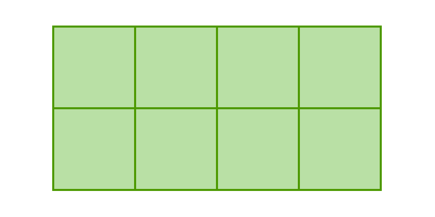\n\n### Augmented Tiling:\n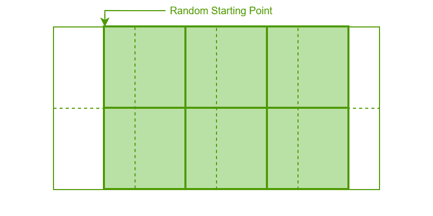\n\nIn augmented data treatment, a sliding starting point is randomly generated during training and from where only 6 tiles are cut out (plus 2 masking tiles) as input. This approach allows the model to see more variations of the image instead of a fixed 8-tile partition. When this approach is used in model structure Type B (tile-level heads) mentioned above, the targets need to be multiplied by 6/8=0.75, because fewer tiles essentially means fewer biomass.\n\nThe probabilty of using augmented tiling in dataloader is set to 0.5, of which the loss weight is set to 0.5 too.\n\n---\n# Training settings\n\nThere are also some standard training settings which are not decisive on their own, but proved to be optimal based on my experience:\n\nTraining are set in two stages, with an early stop patience of 12:\n- In stage 1, only Film layer and heads are trained, with lr starting from 1e-3 down to 2e-5 in 8 epochs\n- In stage 2, backbone is unfreezed, with lr starting from 2e-5 down to 1e-6 in 50 epochs\n\nOther settings:\n\n weight_decay = 0.05\n dropout = 0.3\n loss_w = [0.1, 0.1, 0.1, 0.1, 0.1] # in order of [green, dead, clover, gdm, total], I found this slightly better than [0.1, 0.1, 0.1, 0.2, 0.5] \n\nLoss is computed with huber_loss:\n\n resid = (preds - targets) / scale # (B,5)\n w = torch.tensor(loss_w, device=preds.device, dtype=preds.dtype)\n loss_per_sample = (F.huber_loss(\n resid, torch.zeros_like(resid),\n delta=1.0,\n reduction=\"none\"\n ) * w).sum(dim=1) # (B,)\n\n\n---\n# Submission\n\nI picked two submissions: \n- ensemble of 12 models that I carefully picked with top LB scores (0.75~0.76)\n- ensemble of 26 models with decent LB scores (0.74~0.76).\n\nEvenually both of them achieve a private LB of 0.64. However my best submission is a single model using the techniques I summarized above, which got 0.65 in private LB. Sigh~\n\n\n\n ", "votes": 17 } ], "comments": [], "raw_markdown_by_id": { "3398395": "This has been one of the most frustrating competitions I’ve participated in so far. Everything felt extremely random. I tried countless approaches, but only a handful of them actually worked (or maybe not? 😂). The CV and LB fluctuated unpredictably. In the end, I had no choice but to ensemble everything I had tried - without even knowing whether it truly helped - and hope for minimal shake-up.\n\nNow that the private leaderboard has been revealed, I’ve revisited all my experiments. This finally allows me to gain more confidence in what genuinely worked and what didn’t. I will ignore the many approaches that turned out to be ineffective, and summarize only the useful findings as concisely as possible:\n\n---\n# Model structures\n\nThere are mainly two variations that are eventually included in my ensembles:\n\n### Type A (heads take mean-pooled feature as input):\n\n\n### Type B (heads take tile-level features as input):\n\n\nType A is essentially adopted from public notebooks, where the film layer is the most effective component:\n\n class FiLM(nn.Module):\n def __init__(self, feat_dim):\n super().__init__()\n hidden = max(32, feat_dim // 2)\n self.mlp = nn.Sequential(\n nn.Linear(feat_dim, hidden),\n nn.ReLU(inplace=True),\n nn.Linear(hidden, feat_dim * 2) # output gamma + beta\n )\n def forward(self, context):\n gamma_beta = self.mlp(context)\n return torch.chunk(gamma_beta, 2, dim=1) # (gamma, beta)\n\nI simplified the original approach by discarding techniques such as left–right feature concatenation, which I believe is unnecessary, since there is no inherent left–right structure in the images.\n\nType B, based on my experiments, consistently yields better results on CV and slightly better results on LB. It leverages the intuition that biomass weight can be estimated at the tile level and then aggregated to obtain the final prediction. Compared to Type A, which relies solely on mean-pooled features fed into the prediction heads, Type B allows the heads to capture richer local information, leading to more accurate final results.\n\nIn terms of variations of heads, I tried 3 heads (green, gdm, total), 4 heads (green, clover, gdm, total), and 5 heads. 5 heads gave the worst results. 3 heads and 4 heads are pretty much identical in CV and LB, so I too included both of them in my ensembles.\n\nOverall, my takeaway is that the backbone is what really drives leaderboard performance - ViT Huge > ViT Large > ViT Small. Beyond that, adding more complex structures (attention, gating, mean–max pooling, etc.) doesn’t help at all given the small image size and dataset. Keeping things simple and elegant works best.\n\n---\n# Data augmentation\n\nThis is the most tricky part, I tried countless methods. This is the only way I found slightly impoved my CV and public LB (and private LB as well):\n\n### Typical Tiling:\n\n\n### Augmented Tiling:\n\n\nIn augmented data treatment, a sliding starting point is randomly generated during training and from where only 6 tiles are cut out (plus 2 masking tiles) as input. This approach allows the model to see more variations of the image instead of a fixed 8-tile partition. When this approach is used in model structure Type B (tile-level heads) mentioned above, the targets need to be multiplied by 6/8=0.75, because fewer tiles essentially means fewer biomass.\n\nThe probabilty of using augmented tiling in dataloader is set to 0.5, of which the loss weight is set to 0.5 too.\n\n---\n# Training settings\n\nThere are also some standard training settings which are not decisive on their own, but proved to be optimal based on my experience:\n\nTraining are set in two stages, with an early stop patience of 12:\n- In stage 1, only Film layer and heads are trained, with lr starting from 1e-3 down to 2e-5 in 8 epochs\n- In stage 2, backbone is unfreezed, with lr starting from 2e-5 down to 1e-6 in 50 epochs\n\nOther settings:\n\n weight_decay = 0.05\n dropout = 0.3\n loss_w = [0.1, 0.1, 0.1, 0.1, 0.1] # in order of [green, dead, clover, gdm, total], I found this slightly better than [0.1, 0.1, 0.1, 0.2, 0.5] \n\nLoss is computed with huber_loss:\n\n resid = (preds - targets) / scale # (B,5)\n w = torch.tensor(loss_w, device=preds.device, dtype=preds.dtype)\n loss_per_sample = (F.huber_loss(\n resid, torch.zeros_like(resid),\n delta=1.0,\n reduction=\"none\"\n ) * w).sum(dim=1) # (B,)\n\n\n---\n# Submission\n\nI picked two submissions: \n- ensemble of 12 models that I carefully picked with top LB scores (0.75~0.76)\n- ensemble of 26 models with decent LB scores (0.74~0.76).\n\nEvenually both of them achieve a private LB of 0.64. However my best submission is a single model using the techniques I summarized above, which got 0.65 in private LB. Sigh~\n\n\n\n " } }