
I would first like to thank Kaggle, the sponsors, and the research team for hosting this competition. Initially, it genuinely felt that the dataset was too small. However, as the competition progressed and the leaderboard experienced massive shake-ups, it became clear that this was in fact somehow necessary for the dataset to be small. This was further concluded especially after I got surrounded by Public LB Toppers on Private LB where #1, #2 and #3 on Public LB got #38, #35, #36 on Private LB (respectively) whereas I went from #49 on Public LB to #37 on Private LB, hence surrounded by toppers. The limited data strongly penalized overfitting and forced participants to confront the true generalization ability of their solutions. In hindsight, this constraint was one of the most valuable aspects of the competition.
\nI would also like to express my gratitude to Qiyu Liao for being one of the most active and supportive competition hosts I have seen online on such kaggle competitions. Whether it was clarifying doubts, responding to discussions, or encouraging participants when they share findings openly, your presence significantly elevated the collaborative spirit of the competition. 💙
\nWhen it comes to Clearing doubts, A special mention also goes to PC Jimmy sir as well. When it came to debugging and clearing doubts, you consistently went above and beyond. Entire notebooks were carefully inspected, every issue was addressed, and explanations were delivered with remarkable clarity and patience, often breaking down complex problems to their simplest form. The fact that this was done selflessly and without any expectation of return is deeply inspiring and speaks volumes about the strength of this community. You are a great encouragement showing how supportive a person can really be.
\nBeyond the final solution, I actively shared insights and experimental findings throughout the competition. Two of my discussion posts became the 2nd highest and 5th highest voted discussions in the competition. These focused primarily on clarifying modeling ambiguities, particularly around the Dead Matter target, and on proposing practical strategies to handle its inherent inconsistencies. I believe these discussions helped surface important issues early and encouraged more robust solution design across the community.
\nI experimented with several strong vision backbones, including DINOv2, DINOv3, and EVA02. Among these, EVA02 was particularly interesting during early experimentation because it consistently achieved higher cross-validation scores with less effort compared to both DINOv2 and DINOv3.
\nHowever, despite its promising cross-validation behavior, EVA02 consistently underperformed DINOv3 on the leaderboard. Moreover, models based on DINOv3 exhibited a noticeably smaller gap between training and validation losses. This discrepancy strongly suggested that DINOv3 was learning representations that generalized better beyond the training distribution.
\nThe explanation is largely rooted in the way DINOv3 is trained. Its self-supervised learning objective, combined with its ability to retain rich second-order statistics through Gram matrix information, makes it exceptionally well-suited for dense prediction and regression-style tasks. In the context of this competition, where subtle spatial cues matter more than explicit semantic categories, this property turned out to be crucial.
\nAfter experimenting with many architectural variants, the final model was built around Visual Prompt Tuning combined with DETR-style query tokens, which I refer to here as task tokens.
\nIn addition to the standard image patch embeddings, I appended two types of learnable tokens to the input of DINOv3. The first type consisted of four task tokens, one for each target variable, with the Dead target being derived. The second type consisted of sixteen prompt tokens intended to guide the backbone toward task-relevant representations.
\nDuring the forward pass, all tokens were processed jointly by the backbone. From the output, I extracted the task token embedding corresponding to each target, along with global average pooled and standard deviation pooled features from the patch tokens. These representations were concatenated and passed through target-specific heads to produce the final predictions. Note that each Target head only received its corresponding Task token with GAP and STD, not the other task tokens.
\n
While monitoring training dynamics, I observed that both task tokens and prompt tokens gradually converged toward very similar representations. This collapse significantly reduced the effectiveness of having multiple tokens in the first place.
\nTo counteract this, I introduced an explicit orthogonality loss that encouraged tokens to remain decorrelated. This ensured that each token focused on capturing distinct aspects of the input rather than redundantly encoding the same information. The addition of this constraint proved critical for stable convergence and improved robustness. You can assume that it performs the same role as that of multi head in MHSA (Multi Head Self Attention).
\nTo further improve convergence, I adopted the idea of Self Prompt Tuning.
\nFor each target variable, I selected the ten training samples with the highest target values. From these samples, I extracted the CLS token embeddings and computed their mean. This mean representation was then used to initialize the corresponding task token. The same procedure was applied to initialize the prompt tokens, where the sixteen prompt tokens were divided into four groups (encouraging 1 group for each target).
\nHowever, this initialization strategy naturally caused a sharp increase in orthogonality loss because all tokens started from correlated representations. To resolve this, I applied Gram Schmidt orthogonalization at initialization time, ensuring that all tokens were mutually orthogonal before training began. This allowed the benefits of informed initialization without sacrificing token diversity.
\nWithin the first month of the competition, I realized that the choice of cross-validation strategy would dominate everything else. I shared this insight early on in detail, including implementation specifics, in what later became the most upvoted discussion of the competition. However, the strategy was simply ignored by most.
\nThe initial strategy involved Monte Carlo seed searching combined with GroupKFold splits over both State and Sampling Date, motivated by early speculation that certain states might be entirely absent from the test set. Later clarifications from the competition hosts confirmed that all states were present in the test data, while only specific sites or locations might be unseen. Based on this, I simplified the strategy to state-stratified GroupKFold splits over sampling dates only.
\nEven at an early leaderboard score of around 0.63, the alignment between cross-validation and leaderboard performance was striking. The mean cross-validation R squared score closely matched the leaderboard score, with only minor variance across folds. This alignment persisted throughout the competition and served as a strong signal that the modeling choices were correctly targeting generalizable patterns rather than exploiting validation artifacts.
\nAs the competition progressed, training times increased substantially, while the dataset itself remained extremely small at only 357 images. At the same time, I wanted to exploit a well-known idea popularized by Chris Deotte sir, where models are retrained on the full dataset after estimating the optimal training duration from cross-validation.
\nAlthough this approach is most commonly applied to tabular models such as XGBoost, the underlying principle remains applicable here. I trained models on full dataset without any validation until they reached the mean training loss observed during cross-validation. This approach consistently produced slightly better leaderboard performance compared to ensembling cross-validation models, reinforcing the idea that data efficiency mattered more than validation monitoring in this setting.
\nI experimented extensively with two-stream architectures where the input image was split into two halves. Initially, I concatenated embeddings from each half and passed them jointly to the prediction head. While this worked reasonably well, it increased model complexity and sensitivity to noise.
\nI then moved to a two-stream summation approach, where each half independently produced a prediction and the results were summed. This formulation, however, suffered from a fundamental limitation. There was no supervision signal indicating which half contributed more to the error, and contrastive losses were not directly applicable. Attempts to resolve this using pseudo-labels generated from a strong ensemble did not yield improvements.
\nThe breakthrough came when switching from summation to mean aggregation. In this setup, each stream was forced to predict the biomass of the entire region using only half of the available information. This intentional information bottleneck dramatically improved robustness and significantly reduced the generalization gap between training and validation losses.
\n
At this point, a natural question arose. If the model could already predict the biomass of an entire region while observing only half of the image, how much visual information was it truly relying on?
\nTo investigate this, I trained the model using random crops of size 448 by 448 sampled from the original 1000 by 2000 images. This restricted the model to roughly ten percent of the total image area per forward pass. Despite this severe information bottleneck, the model continued to perform well and achieved leaderboard scores above 0.6, indicating that it was learning global and textural cues rather than memorizing local patterns.
\nI then extended this idea using a multi-crop training strategy. Multiple random crops were sampled per image, predictions were made independently, and their mean was compared against the ground truth to compute the loss. With two crops, an important equilibrium emerged. The training, validation, and leaderboard R squared scores all converged to approximately 0.72. This alignment suggested that the model had effectively stopped overfitting, making validation redundant. At this stage, I transitioned to training on the full dataset without a validation split.
\nThe behavior became surprising as the number of crops increased. The training R squared score rose rapidly, with 3 crops I got a Train R2 of 0.85, yet the validation score remained 0.72. Wait, what? Even when using eight random crops, covering nearly the entire image, the validation performance stayed fixed at around 0.72. This implied that while the model was learning noise, it was not unlearning the truly generalizable features.
\nWhen these models were trained on the full dataset and evaluated on the leaderboard, a clear pattern emerged.
\nTrain R squared to Leaderboard Score Relationship
\n| Train R² | \nLeaderboard Score | \n
|---|---|
| 0.72 | \n0.72 | \n
| 0.80 | \n0.72 | \n
| 0.85 | \n0.73 | \n
| 0.90 | \n0.74 | \n
| 0.92 | \n0.75 | \n
| 0.95 | \n0.75 | \n
Empirically, every increase of roughly 0.05 in training R squared translated to an improvement of about 0.01 on the leaderboard. This counterintuitive effect ultimately shaped my final strategy. Rather than aggressively preventing overfitting, I allowed it in a controlled manner, trusting that the general representations learned through severe information bottlenecking and self-supervised pretraining would remain stable. At this stage, it is worth to again note that I did not even touch the backbone at all.
\n
During inference, each image was divided into tiles of size 500 by 500, hence extracting 8 tiles from 1000x2000 image, from which a central 448 by 448 crop was extracted. Test-time augmentation was limited to simple geometric flips, including horizontal, vertical, and combined flips. No post-processing was applied.
\nFor the final submission, I ensembled multiple checkpoints obtained from the same training run presented above. I also experimented with exponential moving average and stochastic weight averaging. While these techniques improved convergence smoothness, they did not meaningfully raise the performance ceiling.
\nThis solution is the result of continuous experimentation, many failed ideas, and a strong reliance on community-driven learning. I benefited immensely from open discussions, shared insights, and collective debugging. This write-up is one small attempt to give something back to the community.
\nI strongly encourage questions and discussions. The best ideas in this competition emerged through shared curiosity and healthy skepticism, and I hope this contributes to that spirit.
", "messages": [ { "id": "3398398", "postDate": "01/29/2026 04:29:51", "content": "
I would first like to thank Kaggle, the sponsors, and the research team for hosting this competition. Initially, it genuinely felt that the dataset was too small. However, as the competition progressed and the leaderboard experienced massive shake-ups, it became clear that this was in fact somehow necessary for the dataset to be small. This was further concluded especially after I got surrounded by Public LB Toppers on Private LB where #1, #2 and #3 on Public LB got #38, #35, #36 on Private LB (respectively) whereas I went from #49 on Public LB to #37 on Private LB, hence surrounded by toppers. The limited data strongly penalized overfitting and forced participants to confront the true generalization ability of their solutions. In hindsight, this constraint was one of the most valuable aspects of the competition.
\nI would also like to express my gratitude to Qiyu Liao for being one of the most active and supportive competition hosts I have seen online on such kaggle competitions. Whether it was clarifying doubts, responding to discussions, or encouraging participants when they share findings openly, your presence significantly elevated the collaborative spirit of the competition. 💙
\nWhen it comes to Clearing doubts, A special mention also goes to PC Jimmy sir as well. When it came to debugging and clearing doubts, you consistently went above and beyond. Entire notebooks were carefully inspected, every issue was addressed, and explanations were delivered with remarkable clarity and patience, often breaking down complex problems to their simplest form. The fact that this was done selflessly and without any expectation of return is deeply inspiring and speaks volumes about the strength of this community. You are a great encouragement showing how supportive a person can really be.
\nBeyond the final solution, I actively shared insights and experimental findings throughout the competition. Two of my discussion posts became the 2nd highest and 5th highest voted discussions in the competition. These focused primarily on clarifying modeling ambiguities, particularly around the Dead Matter target, and on proposing practical strategies to handle its inherent inconsistencies. I believe these discussions helped surface important issues early and encouraged more robust solution design across the community.
\nI experimented with several strong vision backbones, including DINOv2, DINOv3, and EVA02. Among these, EVA02 was particularly interesting during early experimentation because it consistently achieved higher cross-validation scores with less effort compared to both DINOv2 and DINOv3.
\nHowever, despite its promising cross-validation behavior, EVA02 consistently underperformed DINOv3 on the leaderboard. Moreover, models based on DINOv3 exhibited a noticeably smaller gap between training and validation losses. This discrepancy strongly suggested that DINOv3 was learning representations that generalized better beyond the training distribution.
\nThe explanation is largely rooted in the way DINOv3 is trained. Its self-supervised learning objective, combined with its ability to retain rich second-order statistics through Gram matrix information, makes it exceptionally well-suited for dense prediction and regression-style tasks. In the context of this competition, where subtle spatial cues matter more than explicit semantic categories, this property turned out to be crucial.
\nAfter experimenting with many architectural variants, the final model was built around Visual Prompt Tuning combined with DETR-style query tokens, which I refer to here as task tokens.
\nIn addition to the standard image patch embeddings, I appended two types of learnable tokens to the input of DINOv3. The first type consisted of four task tokens, one for each target variable, with the Dead target being derived. The second type consisted of sixteen prompt tokens intended to guide the backbone toward task-relevant representations.
\nDuring the forward pass, all tokens were processed jointly by the backbone. From the output, I extracted the task token embedding corresponding to each target, along with global average pooled and standard deviation pooled features from the patch tokens. These representations were concatenated and passed through target-specific heads to produce the final predictions. Note that each Target head only received its corresponding Task token with GAP and STD, not the other task tokens.
\n
While monitoring training dynamics, I observed that both task tokens and prompt tokens gradually converged toward very similar representations. This collapse significantly reduced the effectiveness of having multiple tokens in the first place.
\nTo counteract this, I introduced an explicit orthogonality loss that encouraged tokens to remain decorrelated. This ensured that each token focused on capturing distinct aspects of the input rather than redundantly encoding the same information. The addition of this constraint proved critical for stable convergence and improved robustness. You can assume that it performs the same role as that of multi head in MHSA (Multi Head Self Attention).
\nTo further improve convergence, I adopted the idea of Self Prompt Tuning.
\nFor each target variable, I selected the ten training samples with the highest target values. From these samples, I extracted the CLS token embeddings and computed their mean. This mean representation was then used to initialize the corresponding task token. The same procedure was applied to initialize the prompt tokens, where the sixteen prompt tokens were divided into four groups (encouraging 1 group for each target).
\nHowever, this initialization strategy naturally caused a sharp increase in orthogonality loss because all tokens started from correlated representations. To resolve this, I applied Gram Schmidt orthogonalization at initialization time, ensuring that all tokens were mutually orthogonal before training began. This allowed the benefits of informed initialization without sacrificing token diversity.
\nWithin the first month of the competition, I realized that the choice of cross-validation strategy would dominate everything else. I shared this insight early on in detail, including implementation specifics, in what later became the most upvoted discussion of the competition. However, the strategy was simply ignored by most.
\nThe initial strategy involved Monte Carlo seed searching combined with GroupKFold splits over both State and Sampling Date, motivated by early speculation that certain states might be entirely absent from the test set. Later clarifications from the competition hosts confirmed that all states were present in the test data, while only specific sites or locations might be unseen. Based on this, I simplified the strategy to state-stratified GroupKFold splits over sampling dates only.
\nEven at an early leaderboard score of around 0.63, the alignment between cross-validation and leaderboard performance was striking. The mean cross-validation R squared score closely matched the leaderboard score, with only minor variance across folds. This alignment persisted throughout the competition and served as a strong signal that the modeling choices were correctly targeting generalizable patterns rather than exploiting validation artifacts.
\nAs the competition progressed, training times increased substantially, while the dataset itself remained extremely small at only 357 images. At the same time, I wanted to exploit a well-known idea popularized by Chris Deotte sir, where models are retrained on the full dataset after estimating the optimal training duration from cross-validation.
\nAlthough this approach is most commonly applied to tabular models such as XGBoost, the underlying principle remains applicable here. I trained models on full dataset without any validation until they reached the mean training loss observed during cross-validation. This approach consistently produced slightly better leaderboard performance compared to ensembling cross-validation models, reinforcing the idea that data efficiency mattered more than validation monitoring in this setting.
\nI experimented extensively with two-stream architectures where the input image was split into two halves. Initially, I concatenated embeddings from each half and passed them jointly to the prediction head. While this worked reasonably well, it increased model complexity and sensitivity to noise.
\nI then moved to a two-stream summation approach, where each half independently produced a prediction and the results were summed. This formulation, however, suffered from a fundamental limitation. There was no supervision signal indicating which half contributed more to the error, and contrastive losses were not directly applicable. Attempts to resolve this using pseudo-labels generated from a strong ensemble did not yield improvements.
\nThe breakthrough came when switching from summation to mean aggregation. In this setup, each stream was forced to predict the biomass of the entire region using only half of the available information. This intentional information bottleneck dramatically improved robustness and significantly reduced the generalization gap between training and validation losses.
\n
At this point, a natural question arose. If the model could already predict the biomass of an entire region while observing only half of the image, how much visual information was it truly relying on?
\nTo investigate this, I trained the model using random crops of size 448 by 448 sampled from the original 1000 by 2000 images. This restricted the model to roughly ten percent of the total image area per forward pass. Despite this severe information bottleneck, the model continued to perform well and achieved leaderboard scores above 0.6, indicating that it was learning global and textural cues rather than memorizing local patterns.
\nI then extended this idea using a multi-crop training strategy. Multiple random crops were sampled per image, predictions were made independently, and their mean was compared against the ground truth to compute the loss. With two crops, an important equilibrium emerged. The training, validation, and leaderboard R squared scores all converged to approximately 0.72. This alignment suggested that the model had effectively stopped overfitting, making validation redundant. At this stage, I transitioned to training on the full dataset without a validation split.
\nThe behavior became surprising as the number of crops increased. The training R squared score rose rapidly, with 3 crops I got a Train R2 of 0.85, yet the validation score remained 0.72. Wait, what? Even when using eight random crops, covering nearly the entire image, the validation performance stayed fixed at around 0.72. This implied that while the model was learning noise, it was not unlearning the truly generalizable features.
\nWhen these models were trained on the full dataset and evaluated on the leaderboard, a clear pattern emerged.
\nTrain R squared to Leaderboard Score Relationship
\n| Train R² | \nLeaderboard Score | \n
|---|---|
| 0.72 | \n0.72 | \n
| 0.80 | \n0.72 | \n
| 0.85 | \n0.73 | \n
| 0.90 | \n0.74 | \n
| 0.92 | \n0.75 | \n
| 0.95 | \n0.75 | \n
Empirically, every increase of roughly 0.05 in training R squared translated to an improvement of about 0.01 on the leaderboard. This counterintuitive effect ultimately shaped my final strategy. Rather than aggressively preventing overfitting, I allowed it in a controlled manner, trusting that the general representations learned through severe information bottlenecking and self-supervised pretraining would remain stable. At this stage, it is worth to again note that I did not even touch the backbone at all.
\n
During inference, each image was divided into tiles of size 500 by 500, hence extracting 8 tiles from 1000x2000 image, from which a central 448 by 448 crop was extracted. Test-time augmentation was limited to simple geometric flips, including horizontal, vertical, and combined flips. No post-processing was applied.
\nFor the final submission, I ensembled multiple checkpoints obtained from the same training run presented above. I also experimented with exponential moving average and stochastic weight averaging. While these techniques improved convergence smoothness, they did not meaningfully raise the performance ceiling.
\nThis solution is the result of continuous experimentation, many failed ideas, and a strong reliance on community-driven learning. I benefited immensely from open discussions, shared insights, and collective debugging. This write-up is one small attempt to give something back to the community.
\nI strongly encourage questions and discussions. The best ideas in this competition emerged through shared curiosity and healthy skepticism, and I hope this contributes to that spirit.
", "rawMarkdown": "# 🏅 37st Place Solution: **Self Prompt Tuning with DINOv3**\n\n### *Generalization Without Validation or Fine-Tuning*\n\n---\n\n\n\n## 1. Acknowledgements\n\nI would first like to thank Kaggle, the sponsors, and the research team for hosting this competition. Initially, it genuinely felt that the dataset was too small. However, as the competition progressed and the leaderboard experienced massive shake-ups, it became clear that this was in fact somehow necessary for the dataset to be small. This was further concluded especially after I got surrounded by Public LB Toppers on Private LB where #1, #2 and #3 on Public LB got #38, #35, #36 on Private LB (respectively) whereas I went from #49 on Public LB to #37 on Private LB, hence surrounded by toppers. The limited data strongly penalized overfitting and forced participants to confront the true generalization ability of their solutions. In hindsight, this constraint was one of the most valuable aspects of the competition.\n\nI would also like to express my gratitude to Qiyu Liao for being one of the most active and supportive competition hosts I have seen online on such kaggle competitions. Whether it was clarifying doubts, responding to discussions, or encouraging participants when they share findings openly, your presence significantly elevated the collaborative spirit of the competition. 💙\n\nWhen it comes to Clearing doubts, A special mention also goes to PC Jimmy sir as well. When it came to debugging and clearing doubts, you consistently went above and beyond. Entire notebooks were carefully inspected, every issue was addressed, and explanations were delivered with remarkable clarity and patience, often breaking down complex problems to their simplest form. The fact that this was done selflessly and without any expectation of return is deeply inspiring and speaks volumes about the strength of this community. You are a great encouragement showing how supportive a person can really be.\n\n---\n\n### 📌 Community Contribution Note\n\nBeyond the final solution, I actively shared insights and experimental findings throughout the competition. Two of my discussion posts became the **[2nd highest](https://www.kaggle.com/competitions/csiro-biomass/discussion/650736)** and **[5th highest](https://www.kaggle.com/competitions/csiro-biomass/discussion/669012) voted discussions** in the competition. These focused primarily on clarifying modeling ambiguities, particularly around the **Dead Matter target**, and on proposing practical strategies to handle its inherent inconsistencies. I believe these discussions helped surface important issues early and encouraged more robust solution design across the community.\n\n---\n\n## 2. Coming to the Solution now: Backbone Selection and Rationale\n\nI experimented with several strong vision backbones, including DINOv2, DINOv3, and EVA02. Among these, EVA02 was particularly interesting during early experimentation because it consistently achieved higher cross-validation scores with less effort compared to both DINOv2 and DINOv3.\n\nHowever, despite its promising cross-validation behavior, EVA02 consistently underperformed DINOv3 on the leaderboard. Moreover, models based on DINOv3 exhibited a noticeably smaller gap between training and validation losses. This discrepancy strongly suggested that DINOv3 was learning representations that generalized better beyond the training distribution.\n\nThe explanation is largely rooted in the way DINOv3 is trained. Its self-supervised learning objective, combined with its ability to retain rich second-order statistics through Gram matrix information, makes it exceptionally well-suited for dense prediction and regression-style tasks. In the context of this competition, where subtle spatial cues matter more than explicit semantic categories, this property turned out to be crucial.\n\n---\n\n## 3. Model Architecture\n\n#### 📌 Please find the architecture implementation [here](https://www.kaggle.com/code/komilparmar/multicropvptinov3-implementation)\n\n### 3.1 Visual Prompt Tuning with Task Tokens\n\nAfter experimenting with many architectural variants, the final model was built around Visual Prompt Tuning combined with DETR-style query tokens, which I refer to here as task tokens.\n\nIn addition to the standard image patch embeddings, I appended two types of learnable tokens to the input of DINOv3. The first type consisted of four task tokens, one for each target variable, with the Dead target being derived. The second type consisted of sixteen prompt tokens intended to guide the backbone toward task-relevant representations.\n\nDuring the forward pass, all tokens were processed jointly by the backbone. From the output, I extracted the task token embedding corresponding to each target, along with global average pooled and standard deviation pooled features from the patch tokens. These representations were concatenated and passed through target-specific heads to produce the final predictions. Note that each Target head only received its corresponding Task token with GAP and STD, not the other task tokens.\n\n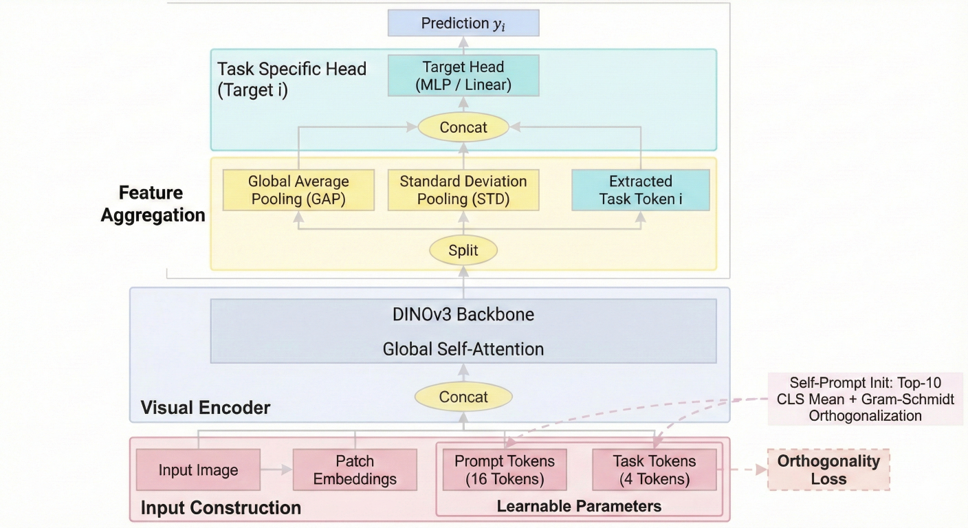\n\n---\n\n### 3.2 Preventing Token Collapse with Orthogonality Loss\n\nWhile monitoring training dynamics, I observed that both task tokens and prompt tokens gradually converged toward very similar representations. This collapse significantly reduced the effectiveness of having multiple tokens in the first place.\n\nTo counteract this, I introduced an explicit orthogonality loss that encouraged tokens to remain decorrelated. This ensured that each token focused on capturing distinct aspects of the input rather than redundantly encoding the same information. The addition of this constraint proved critical for stable convergence and improved robustness. You can assume that it performs the same role as that of multi head in MHSA (Multi Head Self Attention).\n\n---\n\n## 4. Self Prompt Tuning Initialization\n\nTo further improve convergence, I adopted the idea of Self Prompt Tuning.\n\nFor each target variable, I selected the ten training samples with the highest target values. From these samples, I extracted the CLS token embeddings and computed their mean. This mean representation was then used to initialize the corresponding task token. The same procedure was applied to initialize the prompt tokens, where the sixteen prompt tokens were divided into four groups (encouraging 1 group for each target).\n\nHowever, this initialization strategy naturally caused a sharp increase in orthogonality loss because all tokens started from correlated representations. To resolve this, I applied Gram Schmidt orthogonalization at initialization time, ensuring that all tokens were mutually orthogonal before training began. This allowed the benefits of informed initialization without sacrificing token diversity.\n\n---\n\n## 5. Cross-Validation Strategy and Early Generalization Signal\n\nWithin the first month of the competition, I realized that the choice of cross-validation strategy would dominate everything else. I shared this insight early on in detail, including implementation specifics, in what later became the [most upvoted discussion](https://www.kaggle.com/competitions/csiro-biomass/discussion/615401) of the competition. However, the strategy was simply ignored by most.\n\nThe initial strategy involved Monte Carlo seed searching combined with GroupKFold splits over both State and Sampling Date, motivated by early speculation that certain states might be entirely absent from the test set. Later clarifications from the competition hosts confirmed that all states were present in the test data, while only specific sites or locations might be unseen. Based on this, I simplified the strategy to state-stratified GroupKFold splits over sampling dates only.\n\nEven at an early leaderboard score of around 0.63, the alignment between cross-validation and leaderboard performance was striking. The mean cross-validation R squared score closely matched the leaderboard score, with only minor variance across folds. This alignment persisted throughout the competition and served as a strong signal that the modeling choices were correctly targeting generalizable patterns rather than exploiting validation artifacts.\n\n---\n\n## 6. Full Dataset Training Without Validation\n\nAs the competition progressed, training times increased substantially, while the dataset itself remained extremely small at only 357 images. At the same time, I wanted to exploit a well-known idea popularized by Chris Deotte sir, where models are retrained on the full dataset after estimating the optimal training duration from cross-validation.\n\nAlthough this approach is most commonly applied to tabular models such as XGBoost, the underlying principle remains applicable here. I trained models on full dataset without any validation until they reached the mean training loss observed during cross-validation. This approach consistently produced slightly better leaderboard performance compared to ensembling cross-validation models, reinforcing the idea that data efficiency mattered more than validation monitoring in this setting.\n\n---\n\n## 7. From Two-Stream Concat to Mean Aggregation\n\nI experimented extensively with two-stream architectures where the input image was split into two halves. Initially, I concatenated embeddings from each half and passed them jointly to the prediction head. While this worked reasonably well, it increased model complexity and sensitivity to noise.\n\nI then moved to a two-stream summation approach, where each half independently produced a prediction and the results were summed. This formulation, however, suffered from a fundamental limitation. There was no supervision signal indicating which half contributed more to the error, and contrastive losses were not directly applicable. Attempts to resolve this using pseudo-labels generated from a strong ensemble did not yield improvements.\n\nThe breakthrough came when switching from summation to mean aggregation. In this setup, each stream was forced to predict the biomass of the entire region using only half of the available information. This intentional information bottleneck dramatically improved robustness and significantly reduced the generalization gap between training and validation losses.\n\n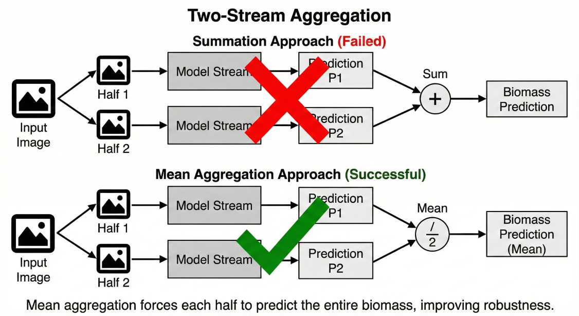\n\n---\n\n## 8. Random Cropping and Information Bottlenecking\n\nAt this point, a natural question arose. If the model could already predict the biomass of an entire region while observing only half of the image, how much visual information was it truly relying on?\n\nTo investigate this, I trained the model using random crops of size 448 by 448 sampled from the original 1000 by 2000 images. This restricted the model to roughly ten percent of the total image area per forward pass. Despite this severe information bottleneck, the model continued to perform well and achieved leaderboard scores above 0.6, indicating that it was learning global and textural cues rather than memorizing local patterns.\n\nI then extended this idea using a multi-crop training strategy. Multiple random crops were sampled per image, predictions were made independently, and their mean was compared against the ground truth to compute the loss. With two crops, an important equilibrium emerged. The training, validation, and leaderboard R squared scores all converged to approximately 0.72. This alignment suggested that the model had effectively stopped overfitting, making validation redundant. At this stage, I transitioned to training on the full dataset without a validation split.\n\nThe behavior became surprising as the number of crops increased. The training R squared score rose rapidly, with 3 crops I got a Train R2 of 0.85, yet the validation score remained 0.72. Wait, what? Even when using eight random crops, covering nearly the entire image, the validation performance stayed fixed at around 0.72. This implied that while the model was learning noise, it was not unlearning the truly generalizable features.\n\nWhen these models were trained on the full dataset and evaluated on the leaderboard, a clear pattern emerged.\n\nTrain R squared to Leaderboard Score Relationship\n\n| Train R² | Leaderboard Score |\n|----------|-------------------|\n| 0.72 | 0.72 |\n| 0.80 | 0.72 |\n| 0.85 | 0.73 |\n| 0.90 | 0.74 |\n| 0.92 | 0.75 |\n| 0.95 | 0.75 |\n\nEmpirically, every increase of roughly 0.05 in training R squared translated to an improvement of about 0.01 on the leaderboard. This counterintuitive effect ultimately shaped my final strategy. Rather than aggressively preventing overfitting, I allowed it in a controlled manner, trusting that the general representations learned through severe information bottlenecking and self-supervised pretraining would remain stable. At this stage, it is worth to again note that I did not even touch the backbone at all.\n\n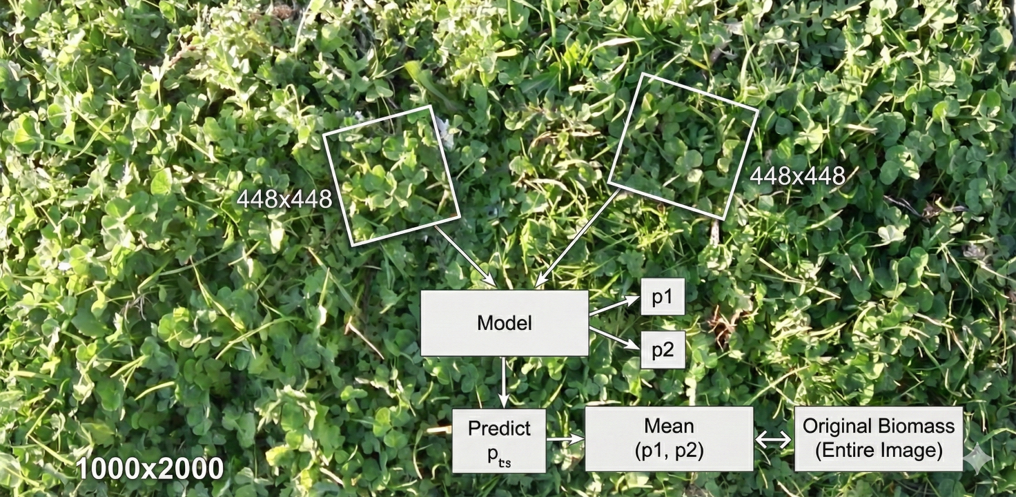\n\n---\n\n## 9. Inference and Ensembling\n\nDuring inference, each image was divided into tiles of size 500 by 500, hence extracting 8 tiles from 1000x2000 image, from which a central 448 by 448 crop was extracted. Test-time augmentation was limited to simple geometric flips, including horizontal, vertical, and combined flips. No post-processing was applied.\n\nFor the final submission, I ensembled multiple checkpoints obtained from the same training run presented above. I also experimented with exponential moving average and stochastic weight averaging. While these techniques improved convergence smoothness, they did not meaningfully raise the performance ceiling.\n\n---\n\n## 10. Conclusion\n\nThis solution is the result of continuous experimentation, many failed ideas, and a strong reliance on community-driven learning. I benefited immensely from open discussions, shared insights, and collective debugging. This write-up is one small attempt to give something back to the community.\n\nI strongly encourage questions and discussions. The best ideas in this competition emerged through shared curiosity and healthy skepticism, and I hope this contributes to that spirit.", "votes": null }, { "id": "3398438", "postDate": "01/29/2026 06:29:12", "content": "I also tried that summation based approch and wasted a lot of time on it it did not worked out at all initially I was summing up the 2D feature map entirely that exploded gradient like crazy. So I implementd a Spatial pooling type of network (simpley defined layer so the spatial map reduced 1x1 using pure conv) that did improve the baseline by 0.02 in LB but still weaker than the simple mean I realized this too late (in fact just 3 days back) as soon as I realized this things moved quickly went from 1200 rank to 208 in public LB
\nAlso maybe training on full dataset might not have been best idea but I get your point, to tackle exact issue I created 3 folds of 66-33 splits. where I sorted the train data by total dry grams and interleaved it so each model saw all spectrum of varitey this was one of my submission
\nby the way great work on your end as well !!! amazing finds
", "rawMarkdown": "I also tried that summation based approch and wasted a lot of time on it it did not worked out at all initially I was summing up the 2D feature map entirely that exploded gradient like crazy. So I implementd a Spatial pooling type of network (simpley defined layer so the spatial map reduced 1x1 using pure conv) that did improve the baseline by 0.02 in LB but still weaker than the simple mean I realized this too late (in fact just 3 days back) as soon as I realized this things moved quickly went from 1200 rank to 208 in public LB\n\nAlso maybe training on full dataset might not have been best idea but I get your point, to tackle exact issue I created 3 folds of 66-33 splits. where I sorted the train data by total dry grams and interleaved it so each model saw all spectrum of varitey this was one of my submission\n\nby the way great work on your end as well !!! amazing finds", "votes": null }, { "id": "3398443", "postDate": "01/29/2026 06:44:45", "content": "Thanks Pushpak. Yes, summing the feature maps entirely will definitely explode the gradients. Even if we do control it, the performance would not be good at all. Because even a tiny change will affect the representation a lot and the heads will not make any sense of it. This is also the reason why SOTA techniques like Mixup and Cutmix didn't hold for this competition for anyone. Because the resultant augmented images made no sense to the image compared to original pure ones. If we instead sum the predictions, even though it too have problems as I explained, we are atleast making sure that the input to the head is consistent, and that the distribution is the same.
\nI tried this same thing with my task tokens recently. I averaged them before passing the heads. But it didn't perform well. It was able to learn correctly, but it overfitted early compared to other runs. The idea was, looking at a single crop, the head should also have a rough idea about the other part of the image, here the other crop, to make better estimations. Turns out, making the heads process/see only its own crop forces it to generate much robust predictions. It also performed better on LB.
", "rawMarkdown": "Thanks Pushpak. Yes, summing the feature maps entirely will definitely explode the gradients. Even if we do control it, the performance would not be good at all. Because even a tiny change will affect the representation a lot and the heads will not make any sense of it. This is also the reason why SOTA techniques like Mixup and Cutmix didn't hold for this competition for anyone. Because the resultant augmented images made no sense to the image compared to original pure ones. If we instead sum the predictions, even though it too have problems as I explained, we are atleast making sure that the input to the head is consistent, and that the distribution is the same. \n\nI tried this same thing with my task tokens recently. I averaged them before passing the heads. But it didn't perform well. It was able to learn correctly, but it overfitted early compared to other runs. The idea was, looking at a single crop, the head should also have a rough idea about the other part of the image, here the other crop, to make better estimations. Turns out, making the heads process/see only its own crop forces it to generate much robust predictions. It also performed better on LB.", "votes": null }, { "id": "3398720", "postDate": "01/29/2026 15:42:33", "content": "Thanks for sharing, I wasn't familiar with some of these techniques, I find them really creative and elegant
", "rawMarkdown": "Thanks for sharing, I wasn't familiar with some of these techniques, I find them really creative and elegant", "votes": null }, { "id": "3398798", "postDate": "01/29/2026 18:01:20", "content": "Thanks @zera12, I am glad the writeup helped.
", "rawMarkdown": "Thanks @zera12, I am glad the writeup helped.", "votes": null }, { "id": "3398805", "postDate": "01/29/2026 18:10:08", "content": "Congrats on your innovative approach! Would you mind sharing your training notebook?
", "rawMarkdown": "Congrats on your innovative approach! Would you mind sharing your training notebook?", "votes": null }, { "id": "3398982", "postDate": "01/30/2026 02:02:34", "content": "Would you mind share your Train R squared to Leaderboard (Public/Private)Score Relationship? Thanks!
", "rawMarkdown": "Would you mind share your Train R squared to Leaderboard (Public/Private)Score Relationship? Thanks!", "votes": null }, { "id": "3399001", "postDate": "01/30/2026 03:20:01", "content": "Thankyou @nacefmbarek. To be honest, the notebook is extremely long and not clean. I may clean it later, add some documentation everywhere, and make a version of it suitable for publishing later. But in the mean time, if you want any specifics, please feel free to ask. Also note that I just shared the architecture implementation here.
", "rawMarkdown": "Thankyou @nacefmbarek. To be honest, the notebook is extremely long and not clean. I may clean it later, add some documentation everywhere, and make a version of it suitable for publishing later. But in the mean time, if you want any specifics, please feel free to ask. Also note that I just shared the architecture implementation [here](https://www.kaggle.com/code/komilparmar/multicropvptinov3-implementation).", "votes": null }, { "id": "3399004", "postDate": "01/30/2026 03:25:17", "content": "Hi @xukongji. I have already shared my Train R2 to Public LB relation above, in section 8. All of those checkpoints are getting 0.62 score on Private LB, while the checkpoints with higher public LB are getting a slightly higher 0.62 score. None of them got 0.63 alone, but their ensemble did.
", "rawMarkdown": "Hi @xukongji. I have already shared my Train R2 to Public LB relation above, in section 8. All of those checkpoints are getting 0.62 score on Private LB, while the checkpoints with higher public LB are getting a slightly higher 0.62 score. None of them got 0.63 alone, but their ensemble did.", "votes": null }, { "id": "3399056", "postDate": "01/30/2026 05:59:13", "content": "Thanks for your response!
", "rawMarkdown": "Thanks for your response!", "votes": null }, { "id": "3402129", "postDate": "02/05/2026 09:41:15", "content": "I found it interesting as well, great job @komilparmar
", "rawMarkdown": "I found it interesting as well, great job @komilparmar", "votes": null }, { "id": "3448805", "postDate": "04/26/2026 16:29:40", "content": "Great work Mr. Parmar \nSpecially the presentation of your Document
", "rawMarkdown": "Great work Mr. Parmar \nSpecially the presentation of your Document", "votes": null } ], "comments": [ { "id": 3398438, "author_name": "pushpakbhoge", "author_url": "", "post_date": "01/29/2026 06:29:12", "content": "I also tried that summation based approch and wasted a lot of time on it it did not worked out at all initially I was summing up the 2D feature map entirely that exploded gradient like crazy. So I implementd a Spatial pooling type of network (simpley defined layer so the spatial map reduced 1x1 using pure conv) that did improve the baseline by 0.02 in LB but still weaker than the simple mean I realized this too late (in fact just 3 days back) as soon as I realized this things moved quickly went from 1200 rank to 208 in public LB
\nAlso maybe training on full dataset might not have been best idea but I get your point, to tackle exact issue I created 3 folds of 66-33 splits. where I sorted the train data by total dry grams and interleaved it so each model saw all spectrum of varitey this was one of my submission
\nby the way great work on your end as well !!! amazing finds
", "votes": null, "replies": [ { "id": 3398443, "author_name": "komilparmar", "author_url": "", "post_date": "01/29/2026 06:44:45", "content": "Thanks Pushpak. Yes, summing the feature maps entirely will definitely explode the gradients. Even if we do control it, the performance would not be good at all. Because even a tiny change will affect the representation a lot and the heads will not make any sense of it. This is also the reason why SOTA techniques like Mixup and Cutmix didn't hold for this competition for anyone. Because the resultant augmented images made no sense to the image compared to original pure ones. If we instead sum the predictions, even though it too have problems as I explained, we are atleast making sure that the input to the head is consistent, and that the distribution is the same.
\nI tried this same thing with my task tokens recently. I averaged them before passing the heads. But it didn't perform well. It was able to learn correctly, but it overfitted early compared to other runs. The idea was, looking at a single crop, the head should also have a rough idea about the other part of the image, here the other crop, to make better estimations. Turns out, making the heads process/see only its own crop forces it to generate much robust predictions. It also performed better on LB.
", "votes": null, "replies": [] } ] }, { "id": 3398720, "author_name": "zera12", "author_url": "", "post_date": "01/29/2026 15:42:33", "content": "Thanks for sharing, I wasn't familiar with some of these techniques, I find them really creative and elegant
", "votes": null, "replies": [ { "id": 3398798, "author_name": "komilparmar", "author_url": "", "post_date": "01/29/2026 18:01:20", "content": "Thanks @zera12, I am glad the writeup helped.
", "votes": null, "replies": [] }, { "id": 3402129, "author_name": "sayidl", "author_url": "", "post_date": "02/05/2026 09:41:15", "content": "I found it interesting as well, great job @komilparmar
", "votes": null, "replies": [] } ] }, { "id": 3398805, "author_name": "nacefmbarek", "author_url": "", "post_date": "01/29/2026 18:10:08", "content": "Congrats on your innovative approach! Would you mind sharing your training notebook?
", "votes": null, "replies": [ { "id": 3399001, "author_name": "komilparmar", "author_url": "", "post_date": "01/30/2026 03:20:01", "content": "Thankyou @nacefmbarek. To be honest, the notebook is extremely long and not clean. I may clean it later, add some documentation everywhere, and make a version of it suitable for publishing later. But in the mean time, if you want any specifics, please feel free to ask. Also note that I just shared the architecture implementation here.
", "votes": null, "replies": [] } ] }, { "id": 3398982, "author_name": "xukongji", "author_url": "", "post_date": "01/30/2026 02:02:34", "content": "Would you mind share your Train R squared to Leaderboard (Public/Private)Score Relationship? Thanks!
", "votes": null, "replies": [ { "id": 3399004, "author_name": "komilparmar", "author_url": "", "post_date": "01/30/2026 03:25:17", "content": "Hi @xukongji. I have already shared my Train R2 to Public LB relation above, in section 8. All of those checkpoints are getting 0.62 score on Private LB, while the checkpoints with higher public LB are getting a slightly higher 0.62 score. None of them got 0.63 alone, but their ensemble did.
", "votes": null, "replies": [ { "id": 3399056, "author_name": "xukongji", "author_url": "", "post_date": "01/30/2026 05:59:13", "content": "Thanks for your response!
", "votes": null, "replies": [] } ] } ] }, { "id": 3448805, "author_name": "trekmac", "author_url": "", "post_date": "04/26/2026 16:29:40", "content": "Great work Mr. Parmar \nSpecially the presentation of your Document
", "votes": null, "replies": [] } ], "raw_markdown_by_id": { "3398398": "# 🏅 37st Place Solution: **Self Prompt Tuning with DINOv3**\n\n### *Generalization Without Validation or Fine-Tuning*\n\n---\n\n\n\n## 1. Acknowledgements\n\nI would first like to thank Kaggle, the sponsors, and the research team for hosting this competition. Initially, it genuinely felt that the dataset was too small. However, as the competition progressed and the leaderboard experienced massive shake-ups, it became clear that this was in fact somehow necessary for the dataset to be small. This was further concluded especially after I got surrounded by Public LB Toppers on Private LB where #1, #2 and #3 on Public LB got #38, #35, #36 on Private LB (respectively) whereas I went from #49 on Public LB to #37 on Private LB, hence surrounded by toppers. The limited data strongly penalized overfitting and forced participants to confront the true generalization ability of their solutions. In hindsight, this constraint was one of the most valuable aspects of the competition.\n\nI would also like to express my gratitude to Qiyu Liao for being one of the most active and supportive competition hosts I have seen online on such kaggle competitions. Whether it was clarifying doubts, responding to discussions, or encouraging participants when they share findings openly, your presence significantly elevated the collaborative spirit of the competition. 💙\n\nWhen it comes to Clearing doubts, A special mention also goes to PC Jimmy sir as well. When it came to debugging and clearing doubts, you consistently went above and beyond. Entire notebooks were carefully inspected, every issue was addressed, and explanations were delivered with remarkable clarity and patience, often breaking down complex problems to their simplest form. The fact that this was done selflessly and without any expectation of return is deeply inspiring and speaks volumes about the strength of this community. You are a great encouragement showing how supportive a person can really be.\n\n---\n\n### 📌 Community Contribution Note\n\nBeyond the final solution, I actively shared insights and experimental findings throughout the competition. Two of my discussion posts became the **[2nd highest](https://www.kaggle.com/competitions/csiro-biomass/discussion/650736)** and **[5th highest](https://www.kaggle.com/competitions/csiro-biomass/discussion/669012) voted discussions** in the competition. These focused primarily on clarifying modeling ambiguities, particularly around the **Dead Matter target**, and on proposing practical strategies to handle its inherent inconsistencies. I believe these discussions helped surface important issues early and encouraged more robust solution design across the community.\n\n---\n\n## 2. Coming to the Solution now: Backbone Selection and Rationale\n\nI experimented with several strong vision backbones, including DINOv2, DINOv3, and EVA02. Among these, EVA02 was particularly interesting during early experimentation because it consistently achieved higher cross-validation scores with less effort compared to both DINOv2 and DINOv3.\n\nHowever, despite its promising cross-validation behavior, EVA02 consistently underperformed DINOv3 on the leaderboard. Moreover, models based on DINOv3 exhibited a noticeably smaller gap between training and validation losses. This discrepancy strongly suggested that DINOv3 was learning representations that generalized better beyond the training distribution.\n\nThe explanation is largely rooted in the way DINOv3 is trained. Its self-supervised learning objective, combined with its ability to retain rich second-order statistics through Gram matrix information, makes it exceptionally well-suited for dense prediction and regression-style tasks. In the context of this competition, where subtle spatial cues matter more than explicit semantic categories, this property turned out to be crucial.\n\n---\n\n## 3. Model Architecture\n\n#### 📌 Please find the architecture implementation [here](https://www.kaggle.com/code/komilparmar/multicropvptinov3-implementation)\n\n### 3.1 Visual Prompt Tuning with Task Tokens\n\nAfter experimenting with many architectural variants, the final model was built around Visual Prompt Tuning combined with DETR-style query tokens, which I refer to here as task tokens.\n\nIn addition to the standard image patch embeddings, I appended two types of learnable tokens to the input of DINOv3. The first type consisted of four task tokens, one for each target variable, with the Dead target being derived. The second type consisted of sixteen prompt tokens intended to guide the backbone toward task-relevant representations.\n\nDuring the forward pass, all tokens were processed jointly by the backbone. From the output, I extracted the task token embedding corresponding to each target, along with global average pooled and standard deviation pooled features from the patch tokens. These representations were concatenated and passed through target-specific heads to produce the final predictions. Note that each Target head only received its corresponding Task token with GAP and STD, not the other task tokens.\n\n\n\n---\n\n### 3.2 Preventing Token Collapse with Orthogonality Loss\n\nWhile monitoring training dynamics, I observed that both task tokens and prompt tokens gradually converged toward very similar representations. This collapse significantly reduced the effectiveness of having multiple tokens in the first place.\n\nTo counteract this, I introduced an explicit orthogonality loss that encouraged tokens to remain decorrelated. This ensured that each token focused on capturing distinct aspects of the input rather than redundantly encoding the same information. The addition of this constraint proved critical for stable convergence and improved robustness. You can assume that it performs the same role as that of multi head in MHSA (Multi Head Self Attention).\n\n---\n\n## 4. Self Prompt Tuning Initialization\n\nTo further improve convergence, I adopted the idea of Self Prompt Tuning.\n\nFor each target variable, I selected the ten training samples with the highest target values. From these samples, I extracted the CLS token embeddings and computed their mean. This mean representation was then used to initialize the corresponding task token. The same procedure was applied to initialize the prompt tokens, where the sixteen prompt tokens were divided into four groups (encouraging 1 group for each target).\n\nHowever, this initialization strategy naturally caused a sharp increase in orthogonality loss because all tokens started from correlated representations. To resolve this, I applied Gram Schmidt orthogonalization at initialization time, ensuring that all tokens were mutually orthogonal before training began. This allowed the benefits of informed initialization without sacrificing token diversity.\n\n---\n\n## 5. Cross-Validation Strategy and Early Generalization Signal\n\nWithin the first month of the competition, I realized that the choice of cross-validation strategy would dominate everything else. I shared this insight early on in detail, including implementation specifics, in what later became the [most upvoted discussion](https://www.kaggle.com/competitions/csiro-biomass/discussion/615401) of the competition. However, the strategy was simply ignored by most.\n\nThe initial strategy involved Monte Carlo seed searching combined with GroupKFold splits over both State and Sampling Date, motivated by early speculation that certain states might be entirely absent from the test set. Later clarifications from the competition hosts confirmed that all states were present in the test data, while only specific sites or locations might be unseen. Based on this, I simplified the strategy to state-stratified GroupKFold splits over sampling dates only.\n\nEven at an early leaderboard score of around 0.63, the alignment between cross-validation and leaderboard performance was striking. The mean cross-validation R squared score closely matched the leaderboard score, with only minor variance across folds. This alignment persisted throughout the competition and served as a strong signal that the modeling choices were correctly targeting generalizable patterns rather than exploiting validation artifacts.\n\n---\n\n## 6. Full Dataset Training Without Validation\n\nAs the competition progressed, training times increased substantially, while the dataset itself remained extremely small at only 357 images. At the same time, I wanted to exploit a well-known idea popularized by Chris Deotte sir, where models are retrained on the full dataset after estimating the optimal training duration from cross-validation.\n\nAlthough this approach is most commonly applied to tabular models such as XGBoost, the underlying principle remains applicable here. I trained models on full dataset without any validation until they reached the mean training loss observed during cross-validation. This approach consistently produced slightly better leaderboard performance compared to ensembling cross-validation models, reinforcing the idea that data efficiency mattered more than validation monitoring in this setting.\n\n---\n\n## 7. From Two-Stream Concat to Mean Aggregation\n\nI experimented extensively with two-stream architectures where the input image was split into two halves. Initially, I concatenated embeddings from each half and passed them jointly to the prediction head. While this worked reasonably well, it increased model complexity and sensitivity to noise.\n\nI then moved to a two-stream summation approach, where each half independently produced a prediction and the results were summed. This formulation, however, suffered from a fundamental limitation. There was no supervision signal indicating which half contributed more to the error, and contrastive losses were not directly applicable. Attempts to resolve this using pseudo-labels generated from a strong ensemble did not yield improvements.\n\nThe breakthrough came when switching from summation to mean aggregation. In this setup, each stream was forced to predict the biomass of the entire region using only half of the available information. This intentional information bottleneck dramatically improved robustness and significantly reduced the generalization gap between training and validation losses.\n\n\n\n---\n\n## 8. Random Cropping and Information Bottlenecking\n\nAt this point, a natural question arose. If the model could already predict the biomass of an entire region while observing only half of the image, how much visual information was it truly relying on?\n\nTo investigate this, I trained the model using random crops of size 448 by 448 sampled from the original 1000 by 2000 images. This restricted the model to roughly ten percent of the total image area per forward pass. Despite this severe information bottleneck, the model continued to perform well and achieved leaderboard scores above 0.6, indicating that it was learning global and textural cues rather than memorizing local patterns.\n\nI then extended this idea using a multi-crop training strategy. Multiple random crops were sampled per image, predictions were made independently, and their mean was compared against the ground truth to compute the loss. With two crops, an important equilibrium emerged. The training, validation, and leaderboard R squared scores all converged to approximately 0.72. This alignment suggested that the model had effectively stopped overfitting, making validation redundant. At this stage, I transitioned to training on the full dataset without a validation split.\n\nThe behavior became surprising as the number of crops increased. The training R squared score rose rapidly, with 3 crops I got a Train R2 of 0.85, yet the validation score remained 0.72. Wait, what? Even when using eight random crops, covering nearly the entire image, the validation performance stayed fixed at around 0.72. This implied that while the model was learning noise, it was not unlearning the truly generalizable features.\n\nWhen these models were trained on the full dataset and evaluated on the leaderboard, a clear pattern emerged.\n\nTrain R squared to Leaderboard Score Relationship\n\n| Train R² | Leaderboard Score |\n|----------|-------------------|\n| 0.72 | 0.72 |\n| 0.80 | 0.72 |\n| 0.85 | 0.73 |\n| 0.90 | 0.74 |\n| 0.92 | 0.75 |\n| 0.95 | 0.75 |\n\nEmpirically, every increase of roughly 0.05 in training R squared translated to an improvement of about 0.01 on the leaderboard. This counterintuitive effect ultimately shaped my final strategy. Rather than aggressively preventing overfitting, I allowed it in a controlled manner, trusting that the general representations learned through severe information bottlenecking and self-supervised pretraining would remain stable. At this stage, it is worth to again note that I did not even touch the backbone at all.\n\n\n\n---\n\n## 9. Inference and Ensembling\n\nDuring inference, each image was divided into tiles of size 500 by 500, hence extracting 8 tiles from 1000x2000 image, from which a central 448 by 448 crop was extracted. Test-time augmentation was limited to simple geometric flips, including horizontal, vertical, and combined flips. No post-processing was applied.\n\nFor the final submission, I ensembled multiple checkpoints obtained from the same training run presented above. I also experimented with exponential moving average and stochastic weight averaging. While these techniques improved convergence smoothness, they did not meaningfully raise the performance ceiling.\n\n---\n\n## 10. Conclusion\n\nThis solution is the result of continuous experimentation, many failed ideas, and a strong reliance on community-driven learning. I benefited immensely from open discussions, shared insights, and collective debugging. This write-up is one small attempt to give something back to the community.\n\nI strongly encourage questions and discussions. The best ideas in this competition emerged through shared curiosity and healthy skepticism, and I hope this contributes to that spirit.", "3398438": "I also tried that summation based approch and wasted a lot of time on it it did not worked out at all initially I was summing up the 2D feature map entirely that exploded gradient like crazy. So I implementd a Spatial pooling type of network (simpley defined layer so the spatial map reduced 1x1 using pure conv) that did improve the baseline by 0.02 in LB but still weaker than the simple mean I realized this too late (in fact just 3 days back) as soon as I realized this things moved quickly went from 1200 rank to 208 in public LB\n\nAlso maybe training on full dataset might not have been best idea but I get your point, to tackle exact issue I created 3 folds of 66-33 splits. where I sorted the train data by total dry grams and interleaved it so each model saw all spectrum of varitey this was one of my submission\n\nby the way great work on your end as well !!! amazing finds", "3398443": "Thanks Pushpak. Yes, summing the feature maps entirely will definitely explode the gradients. Even if we do control it, the performance would not be good at all. Because even a tiny change will affect the representation a lot and the heads will not make any sense of it. This is also the reason why SOTA techniques like Mixup and Cutmix didn't hold for this competition for anyone. Because the resultant augmented images made no sense to the image compared to original pure ones. If we instead sum the predictions, even though it too have problems as I explained, we are atleast making sure that the input to the head is consistent, and that the distribution is the same. \n\nI tried this same thing with my task tokens recently. I averaged them before passing the heads. But it didn't perform well. It was able to learn correctly, but it overfitted early compared to other runs. The idea was, looking at a single crop, the head should also have a rough idea about the other part of the image, here the other crop, to make better estimations. Turns out, making the heads process/see only its own crop forces it to generate much robust predictions. It also performed better on LB.", "3398720": "Thanks for sharing, I wasn't familiar with some of these techniques, I find them really creative and elegant", "3398798": "Thanks @zera12, I am glad the writeup helped.", "3398805": "Congrats on your innovative approach! Would you mind sharing your training notebook?", "3398982": "Would you mind share your Train R squared to Leaderboard (Public/Private)Score Relationship? Thanks!", "3399001": "Thankyou @nacefmbarek. To be honest, the notebook is extremely long and not clean. I may clean it later, add some documentation everywhere, and make a version of it suitable for publishing later. But in the mean time, if you want any specifics, please feel free to ask. Also note that I just shared the architecture implementation [here](https://www.kaggle.com/code/komilparmar/multicropvptinov3-implementation).", "3399004": "Hi @xukongji. I have already shared my Train R2 to Public LB relation above, in section 8. All of those checkpoints are getting 0.62 score on Private LB, while the checkpoints with higher public LB are getting a slightly higher 0.62 score. None of them got 0.63 alone, but their ensemble did.", "3399056": "Thanks for your response!", "3402129": "I found it interesting as well, great job @komilparmar", "3448805": "Great work Mr. Parmar \nSpecially the presentation of your Document" }, "source": "meta" }