
Thanks to the organizers for organizing this competition. It’s been a long time since I last saw a traditional computer vision competition. When this competition first started, I wondered how to tackle the image regression problem besides the traditional techniques I had used before.
\nIn this competition, I use a very simple validation strategy: stratified by State and choosing a seed so that the mean and standard deviation of the labels are similar across all 5 folds. There are a few main reasons: first, the dataset is too small, so if we split it in an extreme way, such as grouping by date or by state, the label distribution would become heavily distorted. Second, the host has confirmed that there are no new species in the public and private test sets. Some states have a certain species while others don’t. Grouping by date also risks missing some species or not having all four seasons represented in the training set. As I understand it, each date group corresponds to a trip to a particular farm to collect samples, and it’s possible that some clover species exist only in certain farms.
\nBasically, my split is almost certainly suffering from data leakage, and I accept that. To mitigate this, I use the CV–LB correlation and the LB score to evaluate the model.
\nRight from the start of the competition, I focused on methods for generating additional training data. However, almost all of my initial experiments failed: the synthetic data, when used to train the model, consistently caused the Public Leaderboard score to drop.\nOne of the main challenges in using synthetic datasets for image regression is the ground truth issue; when an image is modified, the biomass value of each target changes accordingly. To address this, I employed a pseudo-labeling strategy: I used a model trained on the original training set to generate labels for the synthetic dataset, and subsequently trained the final model on the combined dataset (original training set + synthetic dataset).\nI used Qwen Image Edit to create two types of synthetic datasets:
\ntrain_transform = A.ReplayCompose([\n A.RandomResizedCrop(size=(1024, 1024), scale=(0.8, 1.0), interpolation=cv2.INTER_CUBIC, p=1),\n A.HorizontalFlip(p=0.5),\n A.VerticalFlip(p=0.5),\n A.RandomRotate90(p=0.5),\n A.Rotate(limit=(-5, 5), p=0.7),\n A.RandomGamma(gamma_limit=(80, 120), p=0.5),\n A.RandomBrightnessContrast(p=0.75),\n A.HueSaturationValue(hue_shift_limit=10, \n sat_shift_limit=30, \n val_shift_limit=20, p=0.5),\n A.OneOf([\n A.CLAHE(clip_limit=(1, 4), tile_grid_size=(8, 8), p=0.5),\n A.Equalize(p=0.5),\n ], p=0.25),\n A.OneOf([\n A.Sharpen(p=0.5),\n A.Emboss(p=0.5),\n ], p=0.25),\n ])\nFirst, I used these augmentations
\ntrain_transform = A.Compose([\n A.RandomResizedCrop(size=(self.train_imgsize, self.train_imgsize), scale=(0.8, 1.0), interpolation=cv2.INTER_CUBIC, p=1),\n A.HorizontalFlip(p=0.5),\n A.RandomRotate90(p=0.5),\n A.VerticalFlip(p=0.5),\n ])\nAfter that, the augmented images are further processed with RandAugment.
\nrandom_erase = timm.data.random_erasing.RandomErasing(probability=0.5)\nI also used both Mixup and CutMix with α=0.4; both of these augmentations helped improve the CV and public leaderboard scores.\nThe most surprising thing here is that RandomResizedCrop and RandomErasing turned out to play a crucial role in improving both the CV and Public Leaderboard scores. At first, I thought these augmentations would change the image labels and therefore lower the score. But that wasn’t the case. Perhaps the small random crop range reflects the fact that, in reality, the cropped grass region is not always exactly 70×30, but fluctuates slightly around that size.
I used two types of image sizes.
\n| type | \nwidth x height | \n
|---|---|
| 1 | \n2048 x 1024 | \n
| 2 | \n1024 x 1024 | \n
I used Smooth L1 loss. Attempts to use MSE, binary cross-entropy loss, or to apply a log transform to the target values were all unsuccessful.
\ncriterion_green = torch.nn.SmoothL1Loss()\ncriterion_clover = torch.nn.SmoothL1Loss()\ncriterion_dead = torch.nn.SmoothL1Loss()\nI used Schedule-Free Optimizers with layer-wise learning rates
\n| hyper parameters | \nvalue | \n
|---|---|
| lr | \n0.000017 | \n
| batch size | \n2 | \n
| weight decay | \n0.02 | \n
| number of epochs | \n35 | \n
backbone_params = [p for p in model.model.parameters() if p.requires_grad]\nbackbone_ids = set(map(id, backbone_params))\n\n# Identify other parameters\nother_params = [p for p in model.parameters() if p.requires_grad and id(p) not in backbone_ids]\n\nparam_groups = []\nif backbone_params:\n param_groups.append({\n 'params': backbone_params,\n 'lr': 1e-5,\n 'weight_decay': configs['weight_decay'],\n })\nif other_params:\n param_groups.append({\n 'params': other_params,\n 'lr': configs['lr'],\n 'weight_decay': configs['weight_decay'],\n })\noptimizer = schedulefree.AdamWScheduleFree(param_groups, warmup_steps=0)\nMy model predicts three targets: clover, dead, and green. Attempts using 5 targets clover, dead, green, total, gdm and using 3 targets clover, total, gdm both resulted in lower public scores.
\n| backbone | \nselected epoch | \n
|---|---|
| dinov3 vitlarge | \n24-26 | \n
| dinov3 vithuge | \n33-34 | \n
The high-resolution dense features of DINOv3 are truly remarkable. In density estimation tasks, detailed features with high discriminative power are crucial. I experimented with various backbones, including modern ones like dinov2, XCiT, SigLIP, and PE spatial (Perception Encoder), but both CV and LB scores were significantly lower compared to DINOv3.\nAlthough I wanted to ensure diversity, I could only select backbones from DINOv3 family, where ConvNeXt-Large performed significantly worse than ViT-Large.
\nThe idea is that instead of treating this merely as a standard image regression problem, I want to approach it as a density estimation problem. Therefore, I used DINOv3 to extract feature maps of size (N, C, H, W). Then, I tried attaching different heads to estimate the density map. The final results would be the target values for clover, dead, and green.
\n self.model = timm.create_model('vit_large_patch16_dinov3_qkvb.lvd1689m', pretrained=True, features_only=True)\n self.pre_pool_conv = nn.Conv2d(feature_channels, feature_channels, kernel_size=3, padding=1, bias=False)\n self.global_pool = nn.AdaptiveAvgPool2d((1, 1))\n self.reg_head_main = nn.Linear(feature_channels, 3) # clover, dead, green\n def forward(self, x):\n ...\n features = self.model(x)\n last_feature = features[-1]\n last_feature = self.pre_pool_conv(last_feature)\n last_feature = F.relu(last_feature)\n pooled = self.global_pool(last_feature).flatten(1)\n target_values = self.reg_head_main(pooled)\nI wanted to design the model as a semantic segmentation model and found SegDino. By utilizing multiple feature maps and adopting the DPT head from SegDino, I designed the model to output a heatmap where each pixel corresponds to the target value of a 16x16 patch in the image.
\n
...\n self.model = timm.create_model('vit_large_patch16_dinov3_qkvb.lvd1689m', pretrained=True)\n self.feature_indices = [4, 11, 17, 23]\n self.head = DPTHead(3, self.model.embed_dim, 128, False, out_channels=[96, 192, 384, 768])\n\n self.IMAGENET_DEFAULT_MEAN = torch.tensor([0.485, 0.456, 0.406]).to(device_id)\n self.IMAGENET_DEFAULT_STD = torch.tensor([0.229, 0.224, 0.225]).to(device_id)\n\n self.global_pool = nn.AdaptiveAvgPool2d((1, 1))\n\n def forward(self, x, return_features=False):\n ...\n w = x.shape[3]\n x_l = x[:,:,:,:w//2]\n x_r = x[:,:,:,w//2:]\n outputs_l, features_l = self.model.forward_intermediates(x_l, indices=self.feature_indices)\n outputs_r, features_r = self.model.forward_intermediates(x_r, indices=self.feature_indices)\n features_l = self.head(features_l)\n features_r = self.head(features_r)\n\n main_logits_l = self.global_pool(features_l).flatten(1)\n main_logits_r = self.global_pool(features_r).flatten(1)\n main_logits = main_logits_l + main_logits_r\nI visualized the heatmap for each target. White corresponds to a target value of 0, while darker colors indicate values closer to the maximum. The results look promising.
\n\n\n\nHeatmap of the clover target\n\n
\nHeatmap of the dead target\n\n
\nHeatmap of the green target\n\n
I tried classifying the images by State, and surprisingly the accuracy was over 98%.
\nAt the same time, I also plotted the distribution of the targets by State.
\nLabel Distribution per Target per State\n============================================================\n\nTarget: Dry_Clover_g\n----------------------------------------\n count mean std min 25% 50% 75% max\nState \nNSW 75.0 0.134641 1.166028 0.0 0.000000 0.00000 0.000000 10.0981\nTas 138.0 6.239966 11.614679 0.0 0.000000 1.08390 6.628400 71.7865\nVic 112.0 7.106464 9.571358 0.0 1.406525 4.05135 8.274350 67.8977\nWA 32.0 22.087584 20.214792 0.0 4.302500 15.60500 38.200825 58.8800\n\nTarget: Dry_Dead_g\n----------------------------------------\n count mean std min 25% 50% 75% max\nState \nNSW 75.0 14.203379 15.625313 0.0 2.600000 8.36140 20.898100 83.8407\nTas 138.0 15.231128 12.431224 0.4 6.047525 11.07405 21.062300 58.7479\nVic 112.0 10.113879 8.856831 0.0 3.393400 7.22240 13.375525 38.8581\nWA 32.0 0.000000 0.000000 0.0 0.000000 0.00000 0.000000 0.0000\n\nTarget: Dry_Green_g\n----------------------------------------\n count mean std min 25% 50% 75% max\nState \nNSW 75.0 56.559313 31.228115 7.6 30.224150 53.50000 72.829800 157.9836\nTas 138.0 15.327257 13.107406 0.0 3.953725 12.97535 22.857150 69.6107\nVic 112.0 25.449273 16.016427 3.0 13.882050 21.58675 33.037750 89.7395\nWA 32.0 9.299916 18.789542 0.0 0.000000 0.35000 5.413475 72.1000\nIt’s easy to see that all samples from the state of WA have a dead value of 0. Therefore, I applied a post-processing step, setting the dead value of all samples with wa_prob > 0.75 to 0.
\nwa_prob = state_probs[:, 2]\ndead[wa_prob > 0.75] = 0.0\nIn the final days of the competition, I was stuck at a score in the low 0.76x range. After reading @kevin1742064161 ’s comment, I started to suspect there might be bias in the public dataset, so I tried optimizing a scale factor for each target and for each State. Note that my initial attempts to scale the prediction outputs had failed. Surprisingly, the PB score jumped straight from the 0.76822 to 0.77937. And even more surprisingly, this also held on the private leaderboard, where the private score of the ensemble model improved from 0.66153 to 0.67558.
\n# Public LB optimization: \"WA\": {\"clover\": 1.03->1.0, \"clover\": 1.0->0.97, \"clover\": 0.97->0.90, \"clover\": 0.97->0.95,\"green\": 1.0->0.97, \"dead\": 1.0->0.97->0.90->0.80}\n# Public LB optimization: \"VIC\": {\"clover\": 1.0->0.97->0.90, \"clover\": 0.97->0.90}\n# Public LB optimization: \"TAS\": {\"clover\": 0.97->1.0, \"green\": 0.97->1.0}\n# Public LB optimization: \"NSW\": {\"clover\": 0.97->1.0, \"green\": 1.0->1.03}\nSTATE_TARGET_SCALE = {\n \"NSW\": {\"clover\": 1.0, \"dead\": 1.0, \"green\": 1.03},\n \"Tas\": {\"clover\": 1.0, \"dead\": 1.0, \"green\": 1},\n \"Vic\": {\"clover\": 0.85, \"dead\": 1, \"green\": 1},\n \"WA\": {\"clover\": 0.80, \"dead\": 0.80, \"green\": 0.97},\n}\nUse np.clip to restrict the values of the clover, dead, and green variables to specific ranges. The maximum value computed from the training set.
\nclover = np.clip(clover, 0, 71.7865)\ndead = np.clip(dead, 0, 83.8407)\ngreen = np.clip(green, 0, 157.9836)\nDuring training, I noticed that the green target usually converged very early and then started to overfit. The RMSE of the green target typically decreased until around epochs 11–15, and then kept increasing. The remaining targets, clover and dead, usually converged later, around epochs 24–30.\nTherefore, I used the model at epoch 15 to predict the green target, and the model at epoch 26 to predict the other two targets, clover and dead.
\n| Version | \nPublic leaderboard | \nPrivate leaderboard | \n
|---|---|---|
| With the seperate target models | \n0.76731 | \n0.65615 | \n
| Without the seperate target models | \n0.76128 | \n0.64744 | \n
| Model | \nImage size | \nBackbone | \nPublic leaderboard | \nPrivate leaderboard | \n
|---|---|---|---|---|
| conv_relu + 1 tiles | \n2048x1024 | \ndinov3 vit large | \n0.75401 | \n0.63349 | \n
| dpt_head + 1 tiles | \n2048x1024 | \ndinov3 vit large | \n0.75844 | \n0.62890 | \n
| conv_relu + 1 tiles | \n1280x1280 | \ndinov3 vit huge | \n0.75390 | \n0.65361 | \n
| dpt_head + 2 tiles | \n2048x1024 | \ndinov3 vit large | \n0.76379 | \n0.64781 | \n
| dpt_head + 8 tiles | \n2048x1024 | \ndinov3 vit large | \n0.75036 | \n0.62650 | \n
| dpt_head + 2 tiles | \n2048x1024 | \ndinov3 vit huge | \n0.75994 | \n0.66569 | \n
| conv_relu + 2 tiles + separate target models | \n2048x1024 | \ndinov3 vit large | \n0.76731 | \n0.65615 | \n
| conv_relu + 2 tiles | \n2048x1024 | \ndinov3 vit huge | \n0.75718 | \n0.66731 | \n
Looking at the table above, we can see that models with a ViT-Large backbone usually have higher public scores, but the models with a ViT-Huge backbone are the ones that achieve higher private scores.
\nSince I wasn’t sure whether the post-processing technique would also work on the private dataset, I submitted two versions: an ensemble model with the post-processing technique, and an ensemble model without the post-processing technique.
\n| Version | \nPublic leaderboard | \nPrivate leaderboard | \n
|---|---|---|
| With the post-processing technique | \n0.77839 | \n0.67558 | \n
| Without the post-processing technique | \n0.76822 | \n0.66153 | \n
The interesting thing here is that the ensemble models actually had a lower private score than a single model: 0.66153 < 0.67156 (without the post-processing technique). I’ve attached the notebook link for the single model with a private score of 0.67156.\nI really had no way of knowing exactly which single model would perform best on the private dataset, so even though the ensemble’s private score wasn’t perfect, it helped me avoid a shake-up. If I had known exactly which single model had the 0.67156 private score, then with the ensemble method + seperate target models and the post-processing technique I could probably have increased the private score to 0.69 😅
\nI used FP16 quantization and ran two processes on two T4 GPUs. As a result, I was able to reduce the inference time from about 2 hours to 27 minutes.
\nThanks to the organizers for organizing this competition. It’s been a long time since I last saw a traditional computer vision competition. When this competition first started, I wondered how to tackle the image regression problem besides the traditional techniques I had used before.
\nIn this competition, I use a very simple validation strategy: stratified by State and choosing a seed so that the mean and standard deviation of the labels are similar across all 5 folds. There are a few main reasons: first, the dataset is too small, so if we split it in an extreme way, such as grouping by date or by state, the label distribution would become heavily distorted. Second, the host has confirmed that there are no new species in the public and private test sets. Some states have a certain species while others don’t. Grouping by date also risks missing some species or not having all four seasons represented in the training set. As I understand it, each date group corresponds to a trip to a particular farm to collect samples, and it’s possible that some clover species exist only in certain farms.
\nBasically, my split is almost certainly suffering from data leakage, and I accept that. To mitigate this, I use the CV–LB correlation and the LB score to evaluate the model.
\nRight from the start of the competition, I focused on methods for generating additional training data. However, almost all of my initial experiments failed: the synthetic data, when used to train the model, consistently caused the Public Leaderboard score to drop.\nOne of the main challenges in using synthetic datasets for image regression is the ground truth issue; when an image is modified, the biomass value of each target changes accordingly. To address this, I employed a pseudo-labeling strategy: I used a model trained on the original training set to generate labels for the synthetic dataset, and subsequently trained the final model on the combined dataset (original training set + synthetic dataset).\nI used Qwen Image Edit to create two types of synthetic datasets:
\ntrain_transform = A.ReplayCompose([\n A.RandomResizedCrop(size=(1024, 1024), scale=(0.8, 1.0), interpolation=cv2.INTER_CUBIC, p=1),\n A.HorizontalFlip(p=0.5),\n A.VerticalFlip(p=0.5),\n A.RandomRotate90(p=0.5),\n A.Rotate(limit=(-5, 5), p=0.7),\n A.RandomGamma(gamma_limit=(80, 120), p=0.5),\n A.RandomBrightnessContrast(p=0.75),\n A.HueSaturationValue(hue_shift_limit=10, \n sat_shift_limit=30, \n val_shift_limit=20, p=0.5),\n A.OneOf([\n A.CLAHE(clip_limit=(1, 4), tile_grid_size=(8, 8), p=0.5),\n A.Equalize(p=0.5),\n ], p=0.25),\n A.OneOf([\n A.Sharpen(p=0.5),\n A.Emboss(p=0.5),\n ], p=0.25),\n ])\nFirst, I used these augmentations
\ntrain_transform = A.Compose([\n A.RandomResizedCrop(size=(self.train_imgsize, self.train_imgsize), scale=(0.8, 1.0), interpolation=cv2.INTER_CUBIC, p=1),\n A.HorizontalFlip(p=0.5),\n A.RandomRotate90(p=0.5),\n A.VerticalFlip(p=0.5),\n ])\nAfter that, the augmented images are further processed with RandAugment.
\nrandom_erase = timm.data.random_erasing.RandomErasing(probability=0.5)\nI also used both Mixup and CutMix with α=0.4; both of these augmentations helped improve the CV and public leaderboard scores.\nThe most surprising thing here is that RandomResizedCrop and RandomErasing turned out to play a crucial role in improving both the CV and Public Leaderboard scores. At first, I thought these augmentations would change the image labels and therefore lower the score. But that wasn’t the case. Perhaps the small random crop range reflects the fact that, in reality, the cropped grass region is not always exactly 70×30, but fluctuates slightly around that size.
I used two types of image sizes.
\n| type | \nwidth x height | \n
|---|---|
| 1 | \n2048 x 1024 | \n
| 2 | \n1024 x 1024 | \n
I used Smooth L1 loss. Attempts to use MSE, binary cross-entropy loss, or to apply a log transform to the target values were all unsuccessful.
\ncriterion_green = torch.nn.SmoothL1Loss()\ncriterion_clover = torch.nn.SmoothL1Loss()\ncriterion_dead = torch.nn.SmoothL1Loss()\nI used Schedule-Free Optimizers with layer-wise learning rates
\n| hyper parameters | \nvalue | \n
|---|---|
| lr | \n0.000017 | \n
| batch size | \n2 | \n
| weight decay | \n0.02 | \n
| number of epochs | \n35 | \n
backbone_params = [p for p in model.model.parameters() if p.requires_grad]\nbackbone_ids = set(map(id, backbone_params))\n\n# Identify other parameters\nother_params = [p for p in model.parameters() if p.requires_grad and id(p) not in backbone_ids]\n\nparam_groups = []\nif backbone_params:\n param_groups.append({\n 'params': backbone_params,\n 'lr': 1e-5,\n 'weight_decay': configs['weight_decay'],\n })\nif other_params:\n param_groups.append({\n 'params': other_params,\n 'lr': configs['lr'],\n 'weight_decay': configs['weight_decay'],\n })\noptimizer = schedulefree.AdamWScheduleFree(param_groups, warmup_steps=0)\nMy model predicts three targets: clover, dead, and green. Attempts using 5 targets clover, dead, green, total, gdm and using 3 targets clover, total, gdm both resulted in lower public scores.
\n| backbone | \nselected epoch | \n
|---|---|
| dinov3 vitlarge | \n24-26 | \n
| dinov3 vithuge | \n33-34 | \n
The high-resolution dense features of DINOv3 are truly remarkable. In density estimation tasks, detailed features with high discriminative power are crucial. I experimented with various backbones, including modern ones like dinov2, XCiT, SigLIP, and PE spatial (Perception Encoder), but both CV and LB scores were significantly lower compared to DINOv3.\nAlthough I wanted to ensure diversity, I could only select backbones from DINOv3 family, where ConvNeXt-Large performed significantly worse than ViT-Large.
\nThe idea is that instead of treating this merely as a standard image regression problem, I want to approach it as a density estimation problem. Therefore, I used DINOv3 to extract feature maps of size (N, C, H, W). Then, I tried attaching different heads to estimate the density map. The final results would be the target values for clover, dead, and green.
\n self.model = timm.create_model('vit_large_patch16_dinov3_qkvb.lvd1689m', pretrained=True, features_only=True)\n self.pre_pool_conv = nn.Conv2d(feature_channels, feature_channels, kernel_size=3, padding=1, bias=False)\n self.global_pool = nn.AdaptiveAvgPool2d((1, 1))\n self.reg_head_main = nn.Linear(feature_channels, 3) # clover, dead, green\n def forward(self, x):\n ...\n features = self.model(x)\n last_feature = features[-1]\n last_feature = self.pre_pool_conv(last_feature)\n last_feature = F.relu(last_feature)\n pooled = self.global_pool(last_feature).flatten(1)\n target_values = self.reg_head_main(pooled)\nI wanted to design the model as a semantic segmentation model and found SegDino. By utilizing multiple feature maps and adopting the DPT head from SegDino, I designed the model to output a heatmap where each pixel corresponds to the target value of a 16x16 patch in the image.
\n
...\n self.model = timm.create_model('vit_large_patch16_dinov3_qkvb.lvd1689m', pretrained=True)\n self.feature_indices = [4, 11, 17, 23]\n self.head = DPTHead(3, self.model.embed_dim, 128, False, out_channels=[96, 192, 384, 768])\n\n self.IMAGENET_DEFAULT_MEAN = torch.tensor([0.485, 0.456, 0.406]).to(device_id)\n self.IMAGENET_DEFAULT_STD = torch.tensor([0.229, 0.224, 0.225]).to(device_id)\n\n self.global_pool = nn.AdaptiveAvgPool2d((1, 1))\n\n def forward(self, x, return_features=False):\n ...\n w = x.shape[3]\n x_l = x[:,:,:,:w//2]\n x_r = x[:,:,:,w//2:]\n outputs_l, features_l = self.model.forward_intermediates(x_l, indices=self.feature_indices)\n outputs_r, features_r = self.model.forward_intermediates(x_r, indices=self.feature_indices)\n features_l = self.head(features_l)\n features_r = self.head(features_r)\n\n main_logits_l = self.global_pool(features_l).flatten(1)\n main_logits_r = self.global_pool(features_r).flatten(1)\n main_logits = main_logits_l + main_logits_r\nI visualized the heatmap for each target. White corresponds to a target value of 0, while darker colors indicate values closer to the maximum. The results look promising.
\n\n\n\nHeatmap of the clover target\n\n
\nHeatmap of the dead target\n\n
\nHeatmap of the green target\n\n
I tried classifying the images by State, and surprisingly the accuracy was over 98%.
\nAt the same time, I also plotted the distribution of the targets by State.
\nLabel Distribution per Target per State\n============================================================\n\nTarget: Dry_Clover_g\n----------------------------------------\n count mean std min 25% 50% 75% max\nState \nNSW 75.0 0.134641 1.166028 0.0 0.000000 0.00000 0.000000 10.0981\nTas 138.0 6.239966 11.614679 0.0 0.000000 1.08390 6.628400 71.7865\nVic 112.0 7.106464 9.571358 0.0 1.406525 4.05135 8.274350 67.8977\nWA 32.0 22.087584 20.214792 0.0 4.302500 15.60500 38.200825 58.8800\n\nTarget: Dry_Dead_g\n----------------------------------------\n count mean std min 25% 50% 75% max\nState \nNSW 75.0 14.203379 15.625313 0.0 2.600000 8.36140 20.898100 83.8407\nTas 138.0 15.231128 12.431224 0.4 6.047525 11.07405 21.062300 58.7479\nVic 112.0 10.113879 8.856831 0.0 3.393400 7.22240 13.375525 38.8581\nWA 32.0 0.000000 0.000000 0.0 0.000000 0.00000 0.000000 0.0000\n\nTarget: Dry_Green_g\n----------------------------------------\n count mean std min 25% 50% 75% max\nState \nNSW 75.0 56.559313 31.228115 7.6 30.224150 53.50000 72.829800 157.9836\nTas 138.0 15.327257 13.107406 0.0 3.953725 12.97535 22.857150 69.6107\nVic 112.0 25.449273 16.016427 3.0 13.882050 21.58675 33.037750 89.7395\nWA 32.0 9.299916 18.789542 0.0 0.000000 0.35000 5.413475 72.1000\nIt’s easy to see that all samples from the state of WA have a dead value of 0. Therefore, I applied a post-processing step, setting the dead value of all samples with wa_prob > 0.75 to 0.
\nwa_prob = state_probs[:, 2]\ndead[wa_prob > 0.75] = 0.0\nIn the final days of the competition, I was stuck at a score in the low 0.76x range. After reading @kevin1742064161 ’s comment, I started to suspect there might be bias in the public dataset, so I tried optimizing a scale factor for each target and for each State. Note that my initial attempts to scale the prediction outputs had failed. Surprisingly, the PB score jumped straight from the 0.76822 to 0.77937. And even more surprisingly, this also held on the private leaderboard, where the private score of the ensemble model improved from 0.66153 to 0.67558.
\n# Public LB optimization: \"WA\": {\"clover\": 1.03->1.0, \"clover\": 1.0->0.97, \"clover\": 0.97->0.90, \"clover\": 0.97->0.95,\"green\": 1.0->0.97, \"dead\": 1.0->0.97->0.90->0.80}\n# Public LB optimization: \"VIC\": {\"clover\": 1.0->0.97->0.90, \"clover\": 0.97->0.90}\n# Public LB optimization: \"TAS\": {\"clover\": 0.97->1.0, \"green\": 0.97->1.0}\n# Public LB optimization: \"NSW\": {\"clover\": 0.97->1.0, \"green\": 1.0->1.03}\nSTATE_TARGET_SCALE = {\n \"NSW\": {\"clover\": 1.0, \"dead\": 1.0, \"green\": 1.03},\n \"Tas\": {\"clover\": 1.0, \"dead\": 1.0, \"green\": 1},\n \"Vic\": {\"clover\": 0.85, \"dead\": 1, \"green\": 1},\n \"WA\": {\"clover\": 0.80, \"dead\": 0.80, \"green\": 0.97},\n}\nUse np.clip to restrict the values of the clover, dead, and green variables to specific ranges. The maximum value computed from the training set.
\nclover = np.clip(clover, 0, 71.7865)\ndead = np.clip(dead, 0, 83.8407)\ngreen = np.clip(green, 0, 157.9836)\nDuring training, I noticed that the green target usually converged very early and then started to overfit. The RMSE of the green target typically decreased until around epochs 11–15, and then kept increasing. The remaining targets, clover and dead, usually converged later, around epochs 24–30.\nTherefore, I used the model at epoch 15 to predict the green target, and the model at epoch 26 to predict the other two targets, clover and dead.
\n| Version | \nPublic leaderboard | \nPrivate leaderboard | \n
|---|---|---|
| With the seperate target models | \n0.76731 | \n0.65615 | \n
| Without the seperate target models | \n0.76128 | \n0.64744 | \n
| Model | \nImage size | \nBackbone | \nPublic leaderboard | \nPrivate leaderboard | \n
|---|---|---|---|---|
| conv_relu + 1 tiles | \n2048x1024 | \ndinov3 vit large | \n0.75401 | \n0.63349 | \n
| dpt_head + 1 tiles | \n2048x1024 | \ndinov3 vit large | \n0.75844 | \n0.62890 | \n
| conv_relu + 1 tiles | \n1280x1280 | \ndinov3 vit huge | \n0.75390 | \n0.65361 | \n
| dpt_head + 2 tiles | \n2048x1024 | \ndinov3 vit large | \n0.76379 | \n0.64781 | \n
| dpt_head + 8 tiles | \n2048x1024 | \ndinov3 vit large | \n0.75036 | \n0.62650 | \n
| dpt_head + 2 tiles | \n2048x1024 | \ndinov3 vit huge | \n0.75994 | \n0.66569 | \n
| conv_relu + 2 tiles + separate target models | \n2048x1024 | \ndinov3 vit large | \n0.76731 | \n0.65615 | \n
| conv_relu + 2 tiles | \n2048x1024 | \ndinov3 vit huge | \n0.75718 | \n0.66731 | \n
Looking at the table above, we can see that models with a ViT-Large backbone usually have higher public scores, but the models with a ViT-Huge backbone are the ones that achieve higher private scores.
\nSince I wasn’t sure whether the post-processing technique would also work on the private dataset, I submitted two versions: an ensemble model with the post-processing technique, and an ensemble model without the post-processing technique.
\n| Version | \nPublic leaderboard | \nPrivate leaderboard | \n
|---|---|---|
| With the post-processing technique | \n0.77839 | \n0.67558 | \n
| Without the post-processing technique | \n0.76822 | \n0.66153 | \n
The interesting thing here is that the ensemble models actually had a lower private score than a single model: 0.66153 < 0.67156 (without the post-processing technique). I’ve attached the notebook link for the single model with a private score of 0.67156.\nI really had no way of knowing exactly which single model would perform best on the private dataset, so even though the ensemble’s private score wasn’t perfect, it helped me avoid a shake-up. If I had known exactly which single model had the 0.67156 private score, then with the ensemble method + seperate target models and the post-processing technique I could probably have increased the private score to 0.69 😅
\nI used FP16 quantization and ran two processes on two T4 GPUs. As a result, I was able to reduce the inference time from about 2 hours to 27 minutes.
\n@qiyuliaocsiro, Mirage: The Illusion of Visual Understanding - https://arxiv.org/html/2603.21687v2 The issue addressed in this paper aligns with the one I want to emphasize in this competition: I attempted to classify the images by State, and surprisingly, the accuracy exceeded 98%. It seems the model is predicting biomass values based on the ground truth distribution. Specifically, the model infers the farm location and season from the images, and then leverages the ground truth distribution to estimate the average biomass value typical for that particular farm and season.
\nThis could be due to the fact that certain features required for prediction are not present in the images. As highlighted in the discussions below, clover or dead matter can be obscured by the grass layer in some images, meaning the visible quantity is less than the actual amount.
\nConsequently, the model is prone to overfitting to the farm locations and the ground truth distribution. This is clearly demonstrated by the shake-up that occurs when the model encounters new farm locations and seasons.
\nThis mirrors the issue presented in the paper. While the model is supposed to extract visual features like crop density and height from the images, its high accuracy on the public leaderboard is likely a result of overfitting to farm locations and the ground truth distribution (mirage effect).
\nThis also explains why the post-processing technique of scaling the target values based on the State works.
", "rawMarkdown": "@qiyuliaocsiro, Mirage: The Illusion of Visual Understanding - https://arxiv.org/html/2603.21687v2 The issue addressed in this paper aligns with the one I want to emphasize in this competition: I attempted to classify the images by State, and surprisingly, the accuracy exceeded 98%. It seems the model is predicting biomass values based on the ground truth distribution. Specifically, the model infers the **farm location** and **season** from the images, and then leverages the **ground truth distribution** to estimate the average biomass value typical for that particular farm and season.\n\nThis could be due to the fact that certain features required for prediction are not present in the images. As highlighted in the discussions below, **clover or dead** matter can be **obscured** by the grass layer in some images, meaning the visible quantity is less than the actual amount.\n- https://www.kaggle.com/competitions/csiro-biomass/discussion/644876\n- https://www.kaggle.com/competitions/csiro-biomass/discussion/665877\n\nConsequently, the model is prone to overfitting to the farm locations and the ground truth distribution. This is clearly demonstrated by the shake-up that occurs when the model encounters new farm locations and seasons.\n\nThis mirrors the issue presented in the paper. While the model is supposed to extract visual features like **crop density and height** from the images, its high accuracy on the public leaderboard is likely a result of overfitting to **farm locations and the ground truth distribution** (**mirage effect**).\n\nThis also explains why the post-processing technique of scaling the target values based on the State works." }, { "id": 3401206, "postDate": "2026-02-03T06:12:07.240Z", "content": "I have made the training source code public after code cleanup.
", "rawMarkdown": "I have made the training source code public after code cleanup." }, { "id": 3400667, "postDate": "2026-02-02T02:57:55.183Z", "content": "brilliant solution especially the use of DPT decoder
", "rawMarkdown": "brilliant solution especially the use of DPT decoder" }, { "id": 3400056, "postDate": "2026-01-31T20:34:33Z", "content": "However, almost all of my initial experiments failed: the synthetic data, when used to train the model, consistently caused the Public Leaderboard score to drop.\nOne of the main challenges in using synthetic datasets for image regression is the ground truth issue; when an image is modified, the biomass value of each target changes accordingly. \nTo address this, I employed a pseudo-labeling strategy: I used a model trained on the original training set to generate labels for the synthetic dataset, and subsequently trained the final model on the combined dataset (original training set + synthetic dataset).\nNice! entirely missed this lol. When generating synthetic images, I had prompted Nano Banana to preserve the biomass but it still worsened the public LB. Will give your pseudo labelling strategy a try. How much gain did it produce?
\nI've realised that after just doing spring/summer/autumn augmentations, the DINO embeddings have a similarity of 0.99x - so I presume they do not affect the score much. Heavy snow augmentation was the only one that was \"signficantly different\" for me.
", "rawMarkdown": "```\nHowever, almost all of my initial experiments failed: the synthetic data, when used to train the model, consistently caused the Public Leaderboard score to drop.\nOne of the main challenges in using synthetic datasets for image regression is the ground truth issue; when an image is modified, the biomass value of each target changes accordingly. \nTo address this, I employed a pseudo-labeling strategy: I used a model trained on the original training set to generate labels for the synthetic dataset, and subsequently trained the final model on the combined dataset (original training set + synthetic dataset).\n```\nNice! entirely missed this lol. When generating synthetic images, I had prompted Nano Banana to preserve the biomass but it still worsened the public LB. Will give your pseudo labelling strategy a try. How much gain did it produce? \n\nI've realised that after just doing spring/summer/autumn augmentations, the DINO embeddings have a similarity of 0.99x - so I presume they do not affect the score much. Heavy snow augmentation was the only one that was \"signficantly different\" for me.", "replies": [ { "id": 3400059, "postDate": "2026-01-31T20:50:13.610Z", "content": "Before using pseudolabels, when I submitted a model trained on a combination of the training and synthetic datasets, the public score would significantly drop. I was stuck in the 0.75 range for a very long time; despite trying numerous methods, I could not surpass the peak 0.75x score I had achieved a month earlier.
\nAfter implementing pseudolabels, the model's score stabilized, and I was able to continue boosting my LB score. Removing all vegetation while preserving the background facilitated the training of weakly supervised semantic segmentation. At the very least, it helped the model identify regions where biomass should be zero.
\nThe labels changed significantly: for instance, in the 'autumn' scenario, green grass turned completely yellow/withered, while in 'rainy' or 'spring' scenarios, the generative model often added grass to the background.
", "rawMarkdown": "Before using pseudolabels, when I submitted a model trained on a combination of the training and synthetic datasets, the public score would significantly drop. I was stuck in the 0.75 range for a very long time; despite trying numerous methods, I could not surpass the peak 0.75x score I had achieved a month earlier.\n\nAfter implementing pseudolabels, the model's score stabilized, and I was able to continue boosting my LB score. Removing all vegetation while preserving the background facilitated the training of weakly supervised semantic segmentation. At the very least, it helped the model identify regions where biomass should be zero.\n\nThe labels changed significantly: for instance, in the 'autumn' scenario, green grass turned completely yellow/withered, while in 'rainy' or 'spring' scenarios, the generative model often added grass to the background." }, { "id": 3400061, "postDate": "2026-01-31T20:54:56.657Z", "content": " \nYou can check folder ID1012260530.
Qwen has a true_cfg_scale parameter. Increasing this parameter leads to more distinct generated images and higher diversity; however, this also makes the original labels less accurate. Think of the synthetic dataset as an unlabeled external dataset that has a distribution quite similar to, but not exactly the same as, the training set.
", "rawMarkdown": "Qwen has a **true_cfg_scale** parameter. Increasing this parameter leads to more distinct generated images and higher diversity; however, this also makes the original labels less accurate. Think of the synthetic dataset as an unlabeled external dataset that has a distribution quite similar to, but not exactly the same as, the training set." }, { "id": 3400068, "postDate": "2026-01-31T21:15:55.233Z", "content": "I noticed that the top 4 solution removes the timestamp. My solution is to retain that bias and teach the model that it is irrelevant, ensuring that for such images, the biomass should be zero. 
Hmm my score worsened with training on pseudo labels of synthetic images or postprocessing
", "rawMarkdown": "Hmm my score worsened with training on pseudo labels of synthetic images or postprocessing" }, { "id": 3400482, "postDate": "2026-02-01T16:02:20.617Z", "content": "I used synthetic data with a 25% probability and background images at a ratio of only 10 out of 357.
", "rawMarkdown": "I used synthetic data with a 25% probability and background images at a ratio of only 10 out of 357." }, { "id": 3400484, "postDate": "2026-02-01T16:04:40.610Z", "content": "Please note that I included background images in the synthetic datasets. However, during training, I separated the background images into a separate processing pipeline and did not pseudolabel them.
", "rawMarkdown": "Please note that I included background images in the synthetic datasets. However, during training, I separated the background images into a separate processing pipeline and did not pseudolabel them." }, { "id": 3400707, "postDate": "2026-02-02T05:24:52.470Z", "content": "I have the public pseudolabels for the synthetic datasets here.
", "rawMarkdown": "I have the public pseudolabels for the synthetic datasets [here](https://www.kaggle.com/datasets/quan0095/csiro-synthetic-labels)." } ] } ] }, { "id": 3399280, "postDate": "2026-01-30T15:02:34.640Z", "content": "How can we even give you a downvote when we’re witnessing a true masterpiece?\nCongratulations—you truly deserve this place.
\nIn my opinion, the strongest point of your work is synthetic data generation.\nOutstanding job and very well executed genuis ideas .. split data and augmentation ..
", "rawMarkdown": "How can we even give you a downvote when we’re witnessing a true masterpiece?\nCongratulations—you truly deserve this place.\n\nIn my opinion, the strongest point of your work is **synthetic data generation**.\nOutstanding job and very well executed genuis ideas .. split data and augmentation .. ", "replies": [ { "id": 3399683, "postDate": "2026-01-31T06:47:28.830Z", "content": "Thanks, I have officially published the solution write-up. The synthetic data looks great. Also, even though it is only weakly supervised semantic segmentation, the heatmap for each target looks very promising.
", "rawMarkdown": "Thanks, I have officially published the solution write-up. The synthetic data looks great. Also, even though it is only weakly supervised semantic segmentation, the heatmap for each target looks very promising.", "votes": 2 } ] }, { "id": 3433765, "postDate": "2026-04-02T05:07:47.393Z", "rawMarkdown": "", "isDeleted": true } ], "comments": [ { "id": 3433771, "author_name": "Quan Vu", "author_url": "", "post_date": "2026-04-02T05:32:13.360000", "content": "@qiyuliaocsiro, Mirage: The Illusion of Visual Understanding - https://arxiv.org/html/2603.21687v2 The issue addressed in this paper aligns with the one I want to emphasize in this competition: I attempted to classify the images by State, and surprisingly, the accuracy exceeded 98%. It seems the model is predicting biomass values based on the ground truth distribution. Specifically, the model infers the farm location and season from the images, and then leverages the ground truth distribution to estimate the average biomass value typical for that particular farm and season.
\nThis could be due to the fact that certain features required for prediction are not present in the images. As highlighted in the discussions below, clover or dead matter can be obscured by the grass layer in some images, meaning the visible quantity is less than the actual amount.
\nConsequently, the model is prone to overfitting to the farm locations and the ground truth distribution. This is clearly demonstrated by the shake-up that occurs when the model encounters new farm locations and seasons.
\nThis mirrors the issue presented in the paper. While the model is supposed to extract visual features like crop density and height from the images, its high accuracy on the public leaderboard is likely a result of overfitting to farm locations and the ground truth distribution (mirage effect).
\nThis also explains why the post-processing technique of scaling the target values based on the State works.
", "votes": 0, "replies": [] }, { "id": 3401206, "author_name": "Quan Vu", "author_url": "", "post_date": "2026-02-03T06:12:07.240000", "content": "I have made the training source code public after code cleanup.
", "votes": 0, "replies": [] }, { "id": 3400667, "author_name": "samu2505", "author_url": "", "post_date": "2026-02-02T02:57:55.183000", "content": "brilliant solution especially the use of DPT decoder
", "votes": 0, "replies": [] }, { "id": 3400056, "author_name": "Geremie Yeo", "author_url": "", "post_date": "2026-01-31T20:34:33", "content": "However, almost all of my initial experiments failed: the synthetic data, when used to train the model, consistently caused the Public Leaderboard score to drop.\nOne of the main challenges in using synthetic datasets for image regression is the ground truth issue; when an image is modified, the biomass value of each target changes accordingly. \nTo address this, I employed a pseudo-labeling strategy: I used a model trained on the original training set to generate labels for the synthetic dataset, and subsequently trained the final model on the combined dataset (original training set + synthetic dataset).\nNice! entirely missed this lol. When generating synthetic images, I had prompted Nano Banana to preserve the biomass but it still worsened the public LB. Will give your pseudo labelling strategy a try. How much gain did it produce?
\nI've realised that after just doing spring/summer/autumn augmentations, the DINO embeddings have a similarity of 0.99x - so I presume they do not affect the score much. Heavy snow augmentation was the only one that was \"signficantly different\" for me.
", "votes": 0, "replies": [ { "id": 3400059, "author_name": "Quan Vu", "author_url": "", "post_date": "2026-01-31T20:50:13.610000", "content": "Before using pseudolabels, when I submitted a model trained on a combination of the training and synthetic datasets, the public score would significantly drop. I was stuck in the 0.75 range for a very long time; despite trying numerous methods, I could not surpass the peak 0.75x score I had achieved a month earlier.
\nAfter implementing pseudolabels, the model's score stabilized, and I was able to continue boosting my LB score. Removing all vegetation while preserving the background facilitated the training of weakly supervised semantic segmentation. At the very least, it helped the model identify regions where biomass should be zero.
\nThe labels changed significantly: for instance, in the 'autumn' scenario, green grass turned completely yellow/withered, while in 'rainy' or 'spring' scenarios, the generative model often added grass to the background.
", "votes": 0, "replies": [] }, { "id": 3400061, "author_name": "Quan Vu", "author_url": "", "post_date": "2026-01-31T20:54:56.657000", "content": "\nYou can check folder ID1012260530.
Qwen has a true_cfg_scale parameter. Increasing this parameter leads to more distinct generated images and higher diversity; however, this also makes the original labels less accurate. Think of the synthetic dataset as an unlabeled external dataset that has a distribution quite similar to, but not exactly the same as, the training set.
", "votes": 0, "replies": [] }, { "id": 3400068, "author_name": "Quan Vu", "author_url": "", "post_date": "2026-01-31T21:15:55.233000", "content": "I noticed that the top 4 solution removes the timestamp. My solution is to retain that bias and teach the model that it is irrelevant, ensuring that for such images, the biomass should be zero.
Hmm my score worsened with training on pseudo labels of synthetic images or postprocessing
", "votes": 0, "replies": [] }, { "id": 3400482, "author_name": "Quan Vu", "author_url": "", "post_date": "2026-02-01T16:02:20.617000", "content": "I used synthetic data with a 25% probability and background images at a ratio of only 10 out of 357.
", "votes": 0, "replies": [] }, { "id": 3400484, "author_name": "Quan Vu", "author_url": "", "post_date": "2026-02-01T16:04:40.610000", "content": "Please note that I included background images in the synthetic datasets. However, during training, I separated the background images into a separate processing pipeline and did not pseudolabel them.
", "votes": 0, "replies": [] }, { "id": 3400707, "author_name": "Quan Vu", "author_url": "", "post_date": "2026-02-02T05:24:52.470000", "content": "I have the public pseudolabels for the synthetic datasets here.
", "votes": 0, "replies": [] } ] } ] }, { "id": 3399280, "author_name": "benkerrouche abdelbasset", "author_url": "", "post_date": "2026-01-30T15:02:34.640000", "content": "How can we even give you a downvote when we’re witnessing a true masterpiece?\nCongratulations—you truly deserve this place.
\nIn my opinion, the strongest point of your work is synthetic data generation.\nOutstanding job and very well executed genuis ideas .. split data and augmentation ..
", "votes": 0, "replies": [ { "id": 3399683, "author_name": "Quan Vu", "author_url": "", "post_date": "2026-01-31T06:47:28.830000", "content": "Thanks, I have officially published the solution write-up. The synthetic data looks great. Also, even though it is only weakly supervised semantic segmentation, the heatmap for each target looks very promising.
", "votes": 2, "replies": [] } ] }, { "id": 3433765, "author_name": "", "author_url": "", "post_date": "2026-04-02T05:07:47.393000", "content": "", "votes": 0, "replies": [] } ], "raw_markdown_by_id": { "3399023": "Thanks to the organizers for organizing this competition. It’s been a long time since I last saw a traditional computer vision competition. When this competition first started, I wondered how to tackle the image regression problem besides the traditional techniques I had used before.\n# 1. Cross-validation strategy\nIn this competition, I use a very simple validation strategy: stratified by State and choosing a seed so that the mean and standard deviation of the labels are similar across all 5 folds. There are a few main reasons: first, the dataset is too small, so if we split it in an extreme way, such as grouping by date or by state, the label distribution would become heavily distorted. Second, the host has confirmed that there are no new species in the public and private test sets. Some states have a certain species while others don’t. Grouping by date also risks missing some species or not having all four seasons represented in the training set. As I understand it, each date group corresponds to a trip to a particular farm to collect samples, and it’s possible that some clover species exist only in certain farms.\n\nBasically, my split is almost certainly suffering from data leakage, and I accept that. To mitigate this, I use the CV–LB correlation and the LB score to evaluate the model.\n# 2. Synthetic dataset\nRight from the start of the competition, I focused on methods for generating additional training data. However, almost all of my initial experiments failed: the synthetic data, when used to train the model, consistently caused the Public Leaderboard score to drop.\nOne of the main challenges in using synthetic datasets for image regression is the ground truth issue; when an image is modified, the biomass value of each target changes accordingly. To address this, I employed a pseudo-labeling strategy: I used a model trained on the original training set to generate labels for the synthetic dataset, and subsequently trained the final model on the combined dataset (original training set + synthetic dataset).\nI used [Qwen Image Edit](https://github.com/QwenLM/Qwen-Image) to create two types of synthetic datasets:\n1. The synthetic dataset was generated by simulating seasonal weather changes and adding artifacts such as gravel and rocks.\n2. I removed all grass vegetation from the images, retaining only the bare soil, and set the target values for clover, dead, and green to 0. These images were then combined with the training dataset to help the model discriminate between biomass-containing regions and non-biomass regions.\n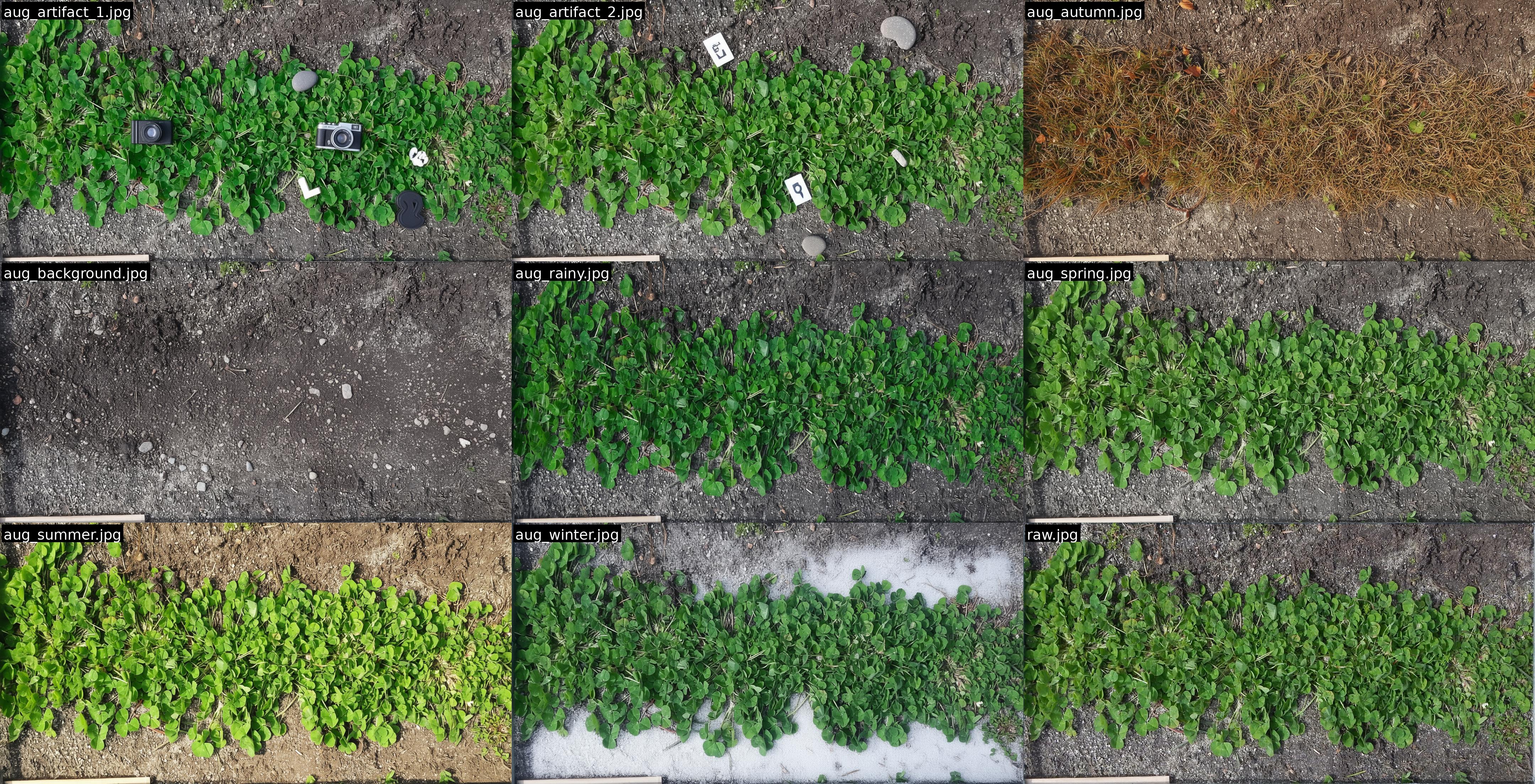\n# 3. Data augmentation\n## Version 1\n```python\ntrain_transform = A.ReplayCompose([\n A.RandomResizedCrop(size=(1024, 1024), scale=(0.8, 1.0), interpolation=cv2.INTER_CUBIC, p=1),\n A.HorizontalFlip(p=0.5),\n A.VerticalFlip(p=0.5),\n A.RandomRotate90(p=0.5),\n A.Rotate(limit=(-5, 5), p=0.7),\n A.RandomGamma(gamma_limit=(80, 120), p=0.5),\n A.RandomBrightnessContrast(p=0.75),\n A.HueSaturationValue(hue_shift_limit=10, \n sat_shift_limit=30, \n val_shift_limit=20, p=0.5),\n A.OneOf([\n A.CLAHE(clip_limit=(1, 4), tile_grid_size=(8, 8), p=0.5),\n A.Equalize(p=0.5),\n ], p=0.25),\n A.OneOf([\n A.Sharpen(p=0.5),\n A.Emboss(p=0.5),\n ], p=0.25),\n ])\n```\n## Version 2\nFirst, I used these augmentations\n```python\ntrain_transform = A.Compose([\n A.RandomResizedCrop(size=(self.train_imgsize, self.train_imgsize), scale=(0.8, 1.0), interpolation=cv2.INTER_CUBIC, p=1),\n A.HorizontalFlip(p=0.5),\n A.RandomRotate90(p=0.5),\n A.VerticalFlip(p=0.5),\n ])\n```\nAfter that, the augmented images are further processed with RandAugment.\n## Other augmentations\n```python\nrandom_erase = timm.data.random_erasing.RandomErasing(probability=0.5)\n```\nI also used both Mixup and CutMix with α=0.4; both of these augmentations helped improve the CV and public leaderboard scores.\nThe most surprising thing here is that `RandomResizedCrop` and `RandomErasing` turned out to play a crucial role in improving both the CV and Public Leaderboard scores. At first, I thought these augmentations would change the image labels and therefore lower the score. But that wasn’t the case. Perhaps the small random crop range reflects the fact that, in reality, the cropped grass region is not always exactly 70×30, but fluctuates slightly around that size.\n## Image size\nI used two types of image sizes.\n| type | width x height |\n| --- | --- |\n| 1| 2048 x 1024 |\n| 2| 1024 x 1024 |\n\n# 4. Optimizing the objective function\n## Loss function\nI used Smooth L1 loss. Attempts to use MSE, binary cross-entropy loss, or to apply a log transform to the target values were all unsuccessful.\n```python\ncriterion_green = torch.nn.SmoothL1Loss()\ncriterion_clover = torch.nn.SmoothL1Loss()\ncriterion_dead = torch.nn.SmoothL1Loss()\n```\n## Optimizer \nI used [Schedule-Free Optimizers](https://github.com/facebookresearch/schedule_free) with layer-wise learning rates\n| hyper parameters | value |\n| --- | --- |\n| lr | 0.000017 |\n| batch size | 2 |\n| weight decay | 0.02 |\n| number of epochs | 35 |\n\n```python\nbackbone_params = [p for p in model.model.parameters() if p.requires_grad]\nbackbone_ids = set(map(id, backbone_params))\n\n# Identify other parameters\nother_params = [p for p in model.parameters() if p.requires_grad and id(p) not in backbone_ids]\n\nparam_groups = []\nif backbone_params:\n param_groups.append({\n 'params': backbone_params,\n 'lr': 1e-5,\n 'weight_decay': configs['weight_decay'],\n })\nif other_params:\n param_groups.append({\n 'params': other_params,\n 'lr': configs['lr'],\n 'weight_decay': configs['weight_decay'],\n })\noptimizer = schedulefree.AdamWScheduleFree(param_groups, warmup_steps=0)\n```\n## The targets \nMy model predicts three targets: **clover**, **dead**, and **green**. Attempts using 5 targets **clover**, **dead**, **green**, **total**, **gdm** and using 3 targets **clover**, **total**, **gdm** both resulted in lower public scores.\n## Early stopping strategy\n| backbone | selected epoch |\n| --- | --- |\n| dinov3 vitlarge | 24-26 |\n| dinov3 vithuge | 33-34 |\n# 5. Model\n## Backbone\nThe high-resolution dense features of DINOv3 are truly remarkable. In density estimation tasks, detailed features with high discriminative power are crucial. I experimented with various backbones, including modern ones like dinov2, XCiT, SigLIP, and PE spatial (Perception Encoder), but both CV and LB scores were significantly lower compared to DINOv3.\nAlthough I wanted to ensure diversity, I could only select backbones from DINOv3 family, where ConvNeXt-Large performed significantly worse than ViT-Large.\n## Weakly supervised semantic segmentation\nThe idea is that instead of treating this merely as a standard image regression problem, I want to approach it as a density estimation problem. Therefore, I used DINOv3 to extract feature maps of size (N, C, H, W). Then, I tried attaching different heads to estimate the density map. The final results would be the target values for clover, dead, and green.\n### First attempt: Simple head Conv + ReLU\n```python\n self.model = timm.create_model('vit_large_patch16_dinov3_qkvb.lvd1689m', pretrained=True, features_only=True)\n self.pre_pool_conv = nn.Conv2d(feature_channels, feature_channels, kernel_size=3, padding=1, bias=False)\n self.global_pool = nn.AdaptiveAvgPool2d((1, 1))\n self.reg_head_main = nn.Linear(feature_channels, 3) # clover, dead, green\n def forward(self, x):\n ...\n features = self.model(x)\n last_feature = features[-1]\n last_feature = self.pre_pool_conv(last_feature)\n last_feature = F.relu(last_feature)\n pooled = self.global_pool(last_feature).flatten(1)\n target_values = self.reg_head_main(pooled)\n```\n### Second attempt: DPT head\nI wanted to design the model as a semantic segmentation model and found [SegDino](https://github.com/script-Yang/SegDINO). By utilizing multiple feature maps and adopting the DPT head from SegDino, I designed the model to output a heatmap where each pixel corresponds to the target value of a 16x16 patch in the image.\n\n#### Backbone\n- Extracts intermediate features at indices [4, 11, 17, 23].\n\n#### DPT Head\n- Projects the 4 input feature maps to [96, 192, 384, 768] channels.\n- Refines them with 3x3 convolutions (\"Scratch\" layers).\n- Upsamples lower-resolution features and concatenates them.\n- Final 1x1 convolution reduces channels to 3 (for the 3 classes).\n\n#### Dual-Path Strategy:\n- The input image is split into left and right halves.\n- Each half is processed independently through the backbone and head.\n- The results are globally pooled and then summed together.\n\n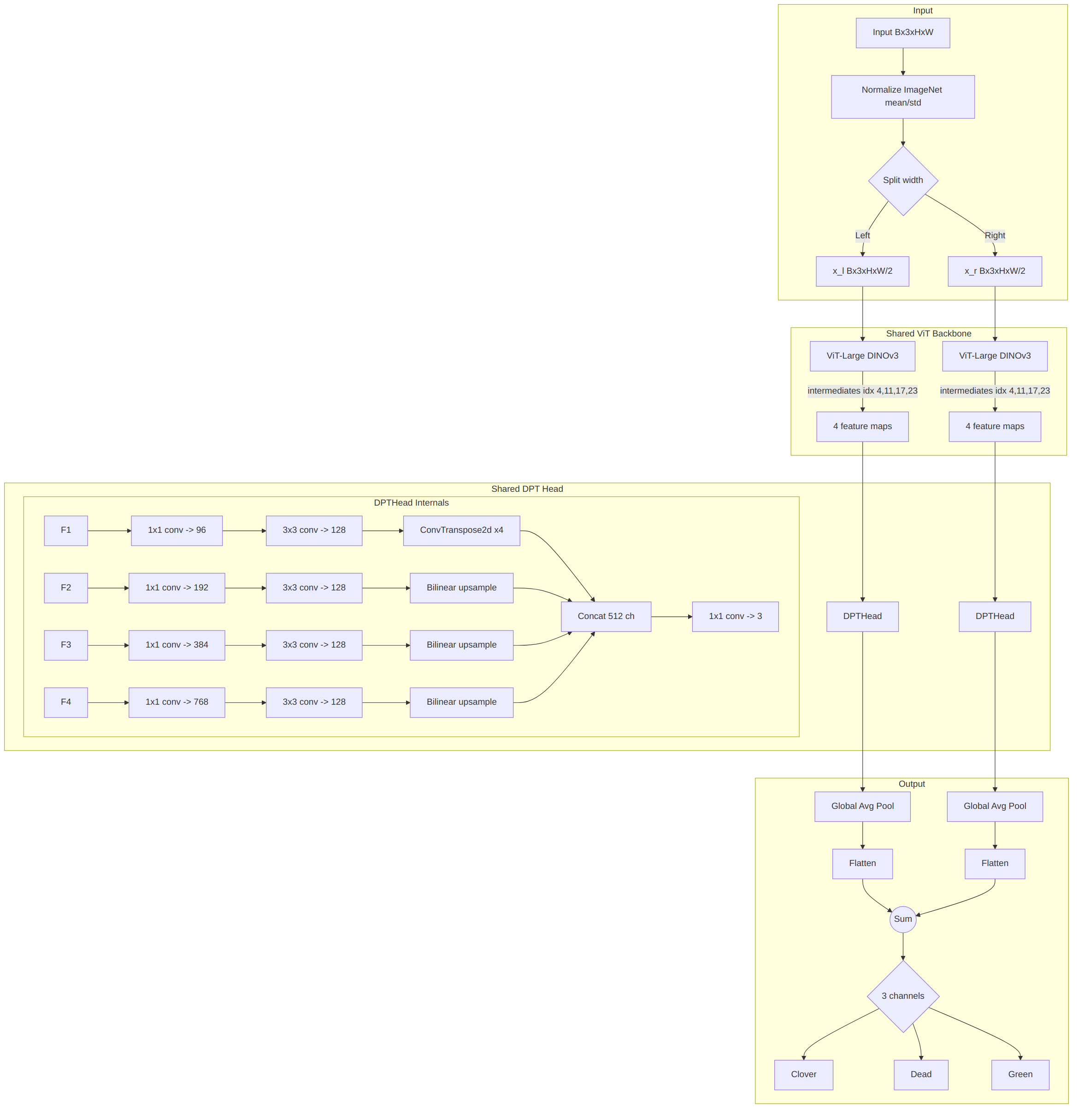\n\n```python\n ...\n self.model = timm.create_model('vit_large_patch16_dinov3_qkvb.lvd1689m', pretrained=True)\n self.feature_indices = [4, 11, 17, 23]\n self.head = DPTHead(3, self.model.embed_dim, 128, False, out_channels=[96, 192, 384, 768])\n\n self.IMAGENET_DEFAULT_MEAN = torch.tensor([0.485, 0.456, 0.406]).to(device_id)\n self.IMAGENET_DEFAULT_STD = torch.tensor([0.229, 0.224, 0.225]).to(device_id)\n\n self.global_pool = nn.AdaptiveAvgPool2d((1, 1))\n\n def forward(self, x, return_features=False):\n ...\n w = x.shape[3]\n x_l = x[:,:,:,:w//2]\n x_r = x[:,:,:,w//2:]\n outputs_l, features_l = self.model.forward_intermediates(x_l, indices=self.feature_indices)\n outputs_r, features_r = self.model.forward_intermediates(x_r, indices=self.feature_indices)\n features_l = self.head(features_l)\n features_r = self.head(features_r)\n\n main_logits_l = self.global_pool(features_l).flatten(1)\n main_logits_r = self.global_pool(features_r).flatten(1)\n main_logits = main_logits_l + main_logits_r\n```\n\nI visualized the heatmap for each target. White corresponds to a target value of 0, while darker colors indicate values closer to the maximum. The results look promising.\n\n> Heatmap of the clover target\n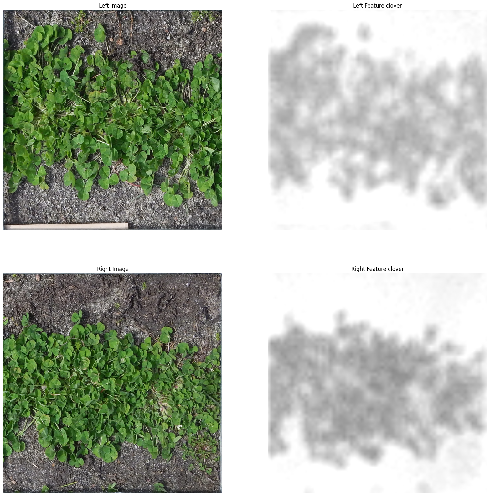\n\n> Heatmap of the dead target\n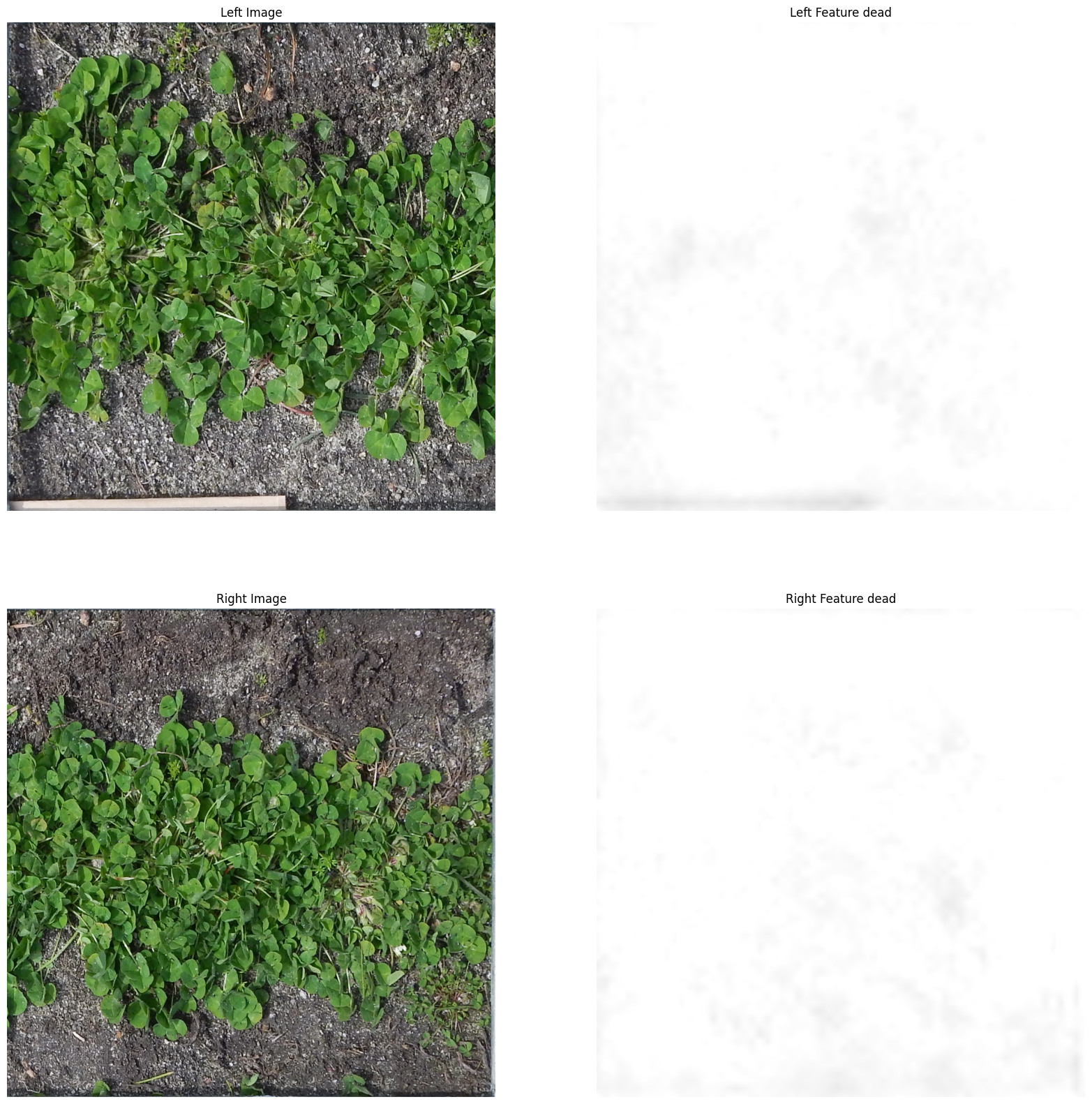\n\n> Heatmap of the green target\n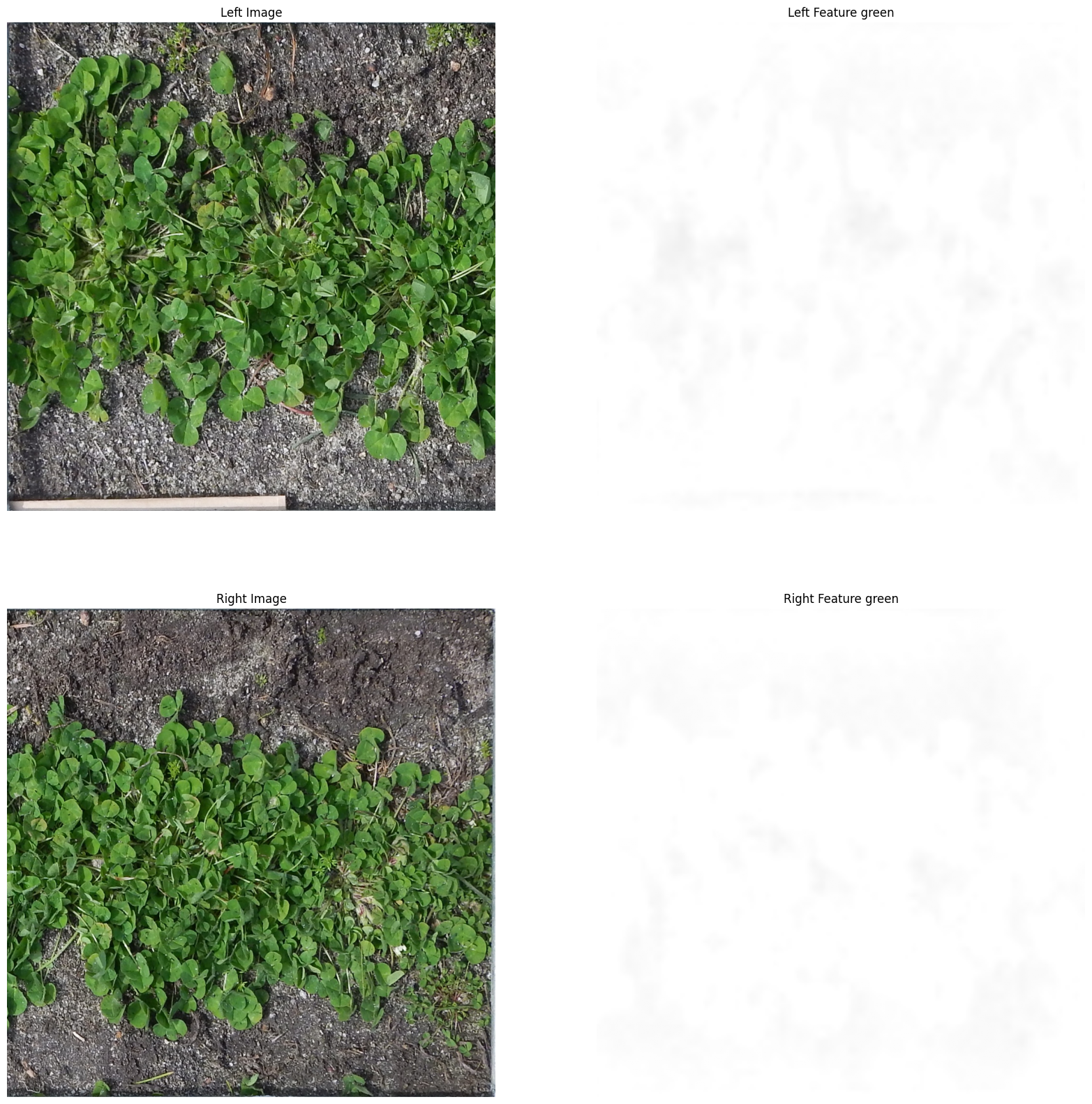\n\n\n# 6. Postprocessing \n\n## State-based scaling postprocess\nI tried classifying the images by State, and surprisingly the accuracy was over 98%.\n\nAt the same time, I also plotted the distribution of the targets by State.\n```bash\nLabel Distribution per Target per State\n============================================================\n\nTarget: Dry_Clover_g\n----------------------------------------\n count mean std min 25% 50% 75% max\nState \nNSW 75.0 0.134641 1.166028 0.0 0.000000 0.00000 0.000000 10.0981\nTas 138.0 6.239966 11.614679 0.0 0.000000 1.08390 6.628400 71.7865\nVic 112.0 7.106464 9.571358 0.0 1.406525 4.05135 8.274350 67.8977\nWA 32.0 22.087584 20.214792 0.0 4.302500 15.60500 38.200825 58.8800\n\nTarget: Dry_Dead_g\n----------------------------------------\n count mean std min 25% 50% 75% max\nState \nNSW 75.0 14.203379 15.625313 0.0 2.600000 8.36140 20.898100 83.8407\nTas 138.0 15.231128 12.431224 0.4 6.047525 11.07405 21.062300 58.7479\nVic 112.0 10.113879 8.856831 0.0 3.393400 7.22240 13.375525 38.8581\nWA 32.0 0.000000 0.000000 0.0 0.000000 0.00000 0.000000 0.0000\n\nTarget: Dry_Green_g\n----------------------------------------\n count mean std min 25% 50% 75% max\nState \nNSW 75.0 56.559313 31.228115 7.6 30.224150 53.50000 72.829800 157.9836\nTas 138.0 15.327257 13.107406 0.0 3.953725 12.97535 22.857150 69.6107\nVic 112.0 25.449273 16.016427 3.0 13.882050 21.58675 33.037750 89.7395\nWA 32.0 9.299916 18.789542 0.0 0.000000 0.35000 5.413475 72.1000\n```\nIt’s easy to see that all samples from the state of WA have a dead value of 0. Therefore, I applied a post-processing step, setting the dead value of all samples with wa_prob > 0.75 to 0.\n```python\nwa_prob = state_probs[:, 2]\ndead[wa_prob > 0.75] = 0.0\n```\nIn the final days of the competition, I was stuck at a score in the low 0.76x range. After reading @kevin1742064161 ’s [comment](https://www.kaggle.com/competitions/csiro-biomass/discussion/668666#3393901), I started to suspect there might be bias in the public dataset, so I tried optimizing a scale factor for each target and for each State. Note that [my initial attempts](https://www.kaggle.com/competitions/csiro-biomass/discussion/665538#3384888) to scale the prediction outputs had failed. Surprisingly, the PB score jumped straight from the 0.76822 to 0.77937. And even more surprisingly, this also held on the private leaderboard, where the private score of the ensemble model improved from 0.66153 to 0.67558.\n```python\n# Public LB optimization: \"WA\": {\"clover\": 1.03->1.0, \"clover\": 1.0->0.97, \"clover\": 0.97->0.90, \"clover\": 0.97->0.95,\"green\": 1.0->0.97, \"dead\": 1.0->0.97->0.90->0.80}\n# Public LB optimization: \"VIC\": {\"clover\": 1.0->0.97->0.90, \"clover\": 0.97->0.90}\n# Public LB optimization: \"TAS\": {\"clover\": 0.97->1.0, \"green\": 0.97->1.0}\n# Public LB optimization: \"NSW\": {\"clover\": 0.97->1.0, \"green\": 1.0->1.03}\nSTATE_TARGET_SCALE = {\n \"NSW\": {\"clover\": 1.0, \"dead\": 1.0, \"green\": 1.03},\n \"Tas\": {\"clover\": 1.0, \"dead\": 1.0, \"green\": 1},\n \"Vic\": {\"clover\": 0.85, \"dead\": 1, \"green\": 1},\n \"WA\": {\"clover\": 0.80, \"dead\": 0.80, \"green\": 0.97},\n}\n```\n\n## Clipping method\nUse np.clip to restrict the values of the clover, dead, and green variables to specific ranges. The maximum value computed from the training set.\n```python\nclover = np.clip(clover, 0, 71.7865)\ndead = np.clip(dead, 0, 83.8407)\ngreen = np.clip(green, 0, 157.9836)\n```\n\n# 7. Inference\n## Seperate target models\nDuring training, I noticed that the green target usually converged very early and then started to overfit. The RMSE of the green target typically decreased until around epochs 11–15, and then kept increasing. The remaining targets, clover and dead, usually converged later, around epochs 24–30.\nTherefore, I used the model at epoch 15 to predict the green target, and the model at epoch 26 to predict the other two targets, clover and dead.\n| Version | Public leaderboard | Private leaderboard |\n| --- | --- | --- |\n| With the seperate target models | **0.76731** | **0.65615** |\n| Without the seperate target models | 0.76128 | 0.64744 |\n\n## List of models used for ensembling\n| Model | Image size| Backbone | Public leaderboard | Private leaderboard |\n| --- | --- | --- | --- | --- |\n| conv_relu + 1 tiles | 2048x1024 | dinov3 vit large | 0.75401 | 0.63349 |\n| dpt_head + 1 tiles | 2048x1024 | dinov3 vit large | 0.75844 | 0.62890 |\n| conv_relu + 1 tiles | 1280x1280 | dinov3 vit huge | 0.75390 | 0.65361 |\n| dpt_head + 2 tiles | 2048x1024 | dinov3 vit large | 0.76379 | 0.64781 |\n| dpt_head + 8 tiles | 2048x1024 | dinov3 vit large | 0.75036 | 0.62650 |\n| dpt_head + 2 tiles | 2048x1024 | dinov3 vit huge | 0.75994 | 0.66569 |\n| conv_relu + 2 tiles + separate target models | 2048x1024 | dinov3 vit large | **0.76731** | 0.65615 |\n| conv_relu + 2 tiles | 2048x1024 | dinov3 vit huge | 0.75718 | **0.66731** |\n\nLooking at the table above, we can see that models with a ViT-Large backbone usually have higher public scores, but the models with a ViT-Huge backbone are the ones that achieve higher private scores.\n## Selection of submissions\nSince I wasn’t sure whether the post-processing technique would also work on the private dataset, I submitted two versions: an ensemble model with the post-processing technique, and an ensemble model without the post-processing technique.\n| Version | Public leaderboard | Private leaderboard |\n| --- | --- | --- |\n| With the post-processing technique| **0.77839** | **0.67558** |\n| Without the post-processing technique| 0.76822 | 0.66153 |\n\nThe interesting thing here is that the ensemble models actually had a lower private score than a single model: 0.66153 < 0.67156 (without the post-processing technique). I’ve attached the notebook link for the single model with a private score of 0.67156.\nI really had no way of knowing exactly which single model would perform best on the private dataset, so even though the ensemble’s private score wasn’t perfect, it helped me avoid a shake-up. If I had known exactly which single model had the 0.67156 private score, then with the ensemble method + seperate target models and the post-processing technique I could probably have increased the private score to 0.69 😅\n\n## Runtime optimization\nI used FP16 quantization and ran two processes on two T4 GPUs. As a result, I was able to reduce the inference time from about **2 hours** to **27 minutes**.\n\n# 8. Trying to find a different approach but without success\n1. Decoding-based Regression: https://www.kaggle.com/competitions/csiro-biomass/discussion/668735\n2. I attempted to use [SAM 2](https://github.com/facebookresearch/sam2) for segmentation. However, since the clover and grass are extremely small and densely intertwined, effective segmentation using SAM 2 proved to be virtually impossible.\n3. I tried using [DiffuseMix](https://github.com/khawar-islam/diffuseMix), but as mentioned earlier, the problem with synthetic data is that when the image changes, the label changes along with it.\n4. Used Excess Green index for segmentation, then used the mask as the 4th channel. Public score did not improve.\n5. Since the biomass estimation problem relies on plant density and height, Height_Ave_cm was used as an auxiliary loss. I also tried using [Depth Anything v3](https://github.com/ByteDance-Seed/Depth-Anything-3) + DINOv3 ViT-Large in a dual-stream model. All methods decreased the public score.\n6. Used Pre_GSHH_NDVI, State, Species, and Height_Ave_cm as auxiliary losses. All resulted in no change or a decrease in the Public score.\n7. Pretrained on an external dataset, then fine-tuned on the training dataset; the public score decreased relatively significantly.\n8. Test time training adaptation: abandoned because it was too time-consuming during inference.\n9. Hflip TTA has no effect or negligible impact with 6-4 weights.", "3433771": "@qiyuliaocsiro, Mirage: The Illusion of Visual Understanding - https://arxiv.org/html/2603.21687v2 The issue addressed in this paper aligns with the one I want to emphasize in this competition: I attempted to classify the images by State, and surprisingly, the accuracy exceeded 98%. It seems the model is predicting biomass values based on the ground truth distribution. Specifically, the model infers the **farm location** and **season** from the images, and then leverages the **ground truth distribution** to estimate the average biomass value typical for that particular farm and season.\n\nThis could be due to the fact that certain features required for prediction are not present in the images. As highlighted in the discussions below, **clover or dead** matter can be **obscured** by the grass layer in some images, meaning the visible quantity is less than the actual amount.\n- https://www.kaggle.com/competitions/csiro-biomass/discussion/644876\n- https://www.kaggle.com/competitions/csiro-biomass/discussion/665877\n\nConsequently, the model is prone to overfitting to the farm locations and the ground truth distribution. This is clearly demonstrated by the shake-up that occurs when the model encounters new farm locations and seasons.\n\nThis mirrors the issue presented in the paper. While the model is supposed to extract visual features like **crop density and height** from the images, its high accuracy on the public leaderboard is likely a result of overfitting to **farm locations and the ground truth distribution** (**mirage effect**).\n\nThis also explains why the post-processing technique of scaling the target values based on the State works.", "3401206": "I have made the training source code public after code cleanup.", "3400667": "brilliant solution especially the use of DPT decoder", "3400056": "```\nHowever, almost all of my initial experiments failed: the synthetic data, when used to train the model, consistently caused the Public Leaderboard score to drop.\nOne of the main challenges in using synthetic datasets for image regression is the ground truth issue; when an image is modified, the biomass value of each target changes accordingly. \nTo address this, I employed a pseudo-labeling strategy: I used a model trained on the original training set to generate labels for the synthetic dataset, and subsequently trained the final model on the combined dataset (original training set + synthetic dataset).\n```\nNice! entirely missed this lol. When generating synthetic images, I had prompted Nano Banana to preserve the biomass but it still worsened the public LB. Will give your pseudo labelling strategy a try. How much gain did it produce? \n\nI've realised that after just doing spring/summer/autumn augmentations, the DINO embeddings have a similarity of 0.99x - so I presume they do not affect the score much. Heavy snow augmentation was the only one that was \"signficantly different\" for me.", "3399280": "How can we even give you a downvote when we’re witnessing a true masterpiece?\nCongratulations—you truly deserve this place.\n\nIn my opinion, the strongest point of your work is **synthetic data generation**.\nOutstanding job and very well executed genuis ideas .. split data and augmentation .. ", "3433765": "" } }

