{"cells":[{"metadata":{},"cell_type":"markdown","source":"# 97% accuracy on MNIST with a single decision tree (+ t-SNE)"},{"metadata":{},"cell_type":"markdown","source":"In this kernel we explore the power of dimensionality reduction for high-dimensional data such as MNIST. We will reduce all 784 pixel features to 2 features and compare the impact it has on the accuracy score. For dimensionality reduction we first use [Truncated Singular Value Decomposition (TSVD)](https://en.wikipedia.org/wiki/Singular_value_decomposition), which is a powerful compression algorithm for matrices such as MNIST digit images. After that we use [t-distributed Stochastic Neighbor Embedding (t-SNE)](https://en.wikipedia.org/wiki/T-distributed_stochastic_neighbor_embedding) on the compressed data from TSVD. Luckily we can easily implement these algorithms thanks to libraries such as [scikit-learn](https://scikit-learn.org/stable/). Let's dive in!\n\nImage: an example of t-SNE results on the MNIST dataset with labels. In this kernel we will create our own t-SNE visualization. [[Source](https://nlml.github.io/in-raw-numpy/in-raw-numpy-t-sne/)]"},{"metadata":{},"cell_type":"markdown","source":"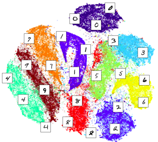![](http://nlml.github.io/images/tsne/tsne-mnist.png)"},{"metadata":{},"cell_type":"markdown","source":"## Table of Contents"},{"metadata":{},"cell_type":"markdown","source":"- [Dependencies](#1)\n- [Preparation](#2)\n- [Metric](#3)\n- [Exploratory Data Analysis (EDA)](#4)\n- [Baseline model](#5)\n- [Dimensionality Reduction (TSVD and t-SNE)](#6)\n- [Modeling](#7)\n- [Evaluation](#8)\n- [Submission](#9)"},{"metadata":{},"cell_type":"markdown","source":"## Dependencies <a id=\"1\"></a>"},{"metadata":{},"cell_type":"markdown","source":"Besides the usual packages we use the library [pydotplus](https://pydotplus.readthedocs.io/). This library provides a Python interface for GraphViz's Dot language and always us to visualize decision trees. Very cool!"},{"metadata":{"_kg_hide-output":true,"_kg_hide-input":false,"trusted":true},"cell_type":"code","source":"# Get the pydotplus package for visualizing decision trees\n!pip install pydotplus","execution_count":null,"outputs":[]},{"metadata":{"_cell_guid":"fd8f7acd-f931-aac7-0d7c-361934322000","trusted":true,"_kg_hide-input":false,"_kg_hide-output":true},"cell_type":"code","source":"# Standard Libraries\nimport os\nimport numpy as np \nimport pandas as pd \nimport random as rn\n\n# Visualization libraries\nimport pydotplus\nimport matplotlib\nimport matplotlib.pyplot as plt\nimport seaborn as sns\nsns.set_style({\"axes.facecolor\": \".95\"})\n\n# Modeling and Machine Learning\nfrom IPython.display import Image \nfrom sklearn.manifold import TSNE\nfrom sklearn.metrics import accuracy_score\nfrom sklearn.externals.six import StringIO  \nfrom sklearn.decomposition import TruncatedSVD\nfrom sklearn.model_selection import train_test_split\nfrom sklearn.tree import DecisionTreeClassifier, export_graphviz\n\n# Specify Paths for easy dataloading\nBASE_PATH = '../input/'\nTRAIN_PATH = BASE_PATH + 'train.csv'\nTEST_PATH = BASE_PATH + 'test.csv'\n\n# Seed for reproducability\nseed = 1234\nnp.random.seed(seed)\nrn.seed(seed)\nos.environ['PYTHONHASHSEED'] = str(seed)","execution_count":null,"outputs":[]},{"metadata":{"_kg_hide-input":true,"trusted":true},"cell_type":"code","source":"# File sizes and specifications\nprint('\\n# Files and file sizes')\nfor file in os.listdir(BASE_PATH):\n    print('{}| {} MB'.format(file.ljust(30), \n                             str(round(os.path.getsize(BASE_PATH + file) / 1000000, 2))))","execution_count":null,"outputs":[]},{"metadata":{},"cell_type":"markdown","source":"## Preparation <a id=\"2\"></a>"},{"metadata":{},"cell_type":"markdown","source":"Loading in files. Note that we concatenate the training and testing data because we would like to train our dimensionality reduction algorithms on all the data we have."},{"metadata":{"_cell_guid":"fb3ee38b-7bf2-d4b7-62ad-3b5b381a84b6","trusted":true,"_kg_hide-output":true,"_kg_hide-input":true},"cell_type":"code","source":"# Load in training and testing data\ntrain_df = pd.read_csv(TRAIN_PATH)\ntest_df = pd.read_csv(TEST_PATH)\nconcat_df = pd.concat([train_df, test_df])\nsample_sub = pd.read_csv(BASE_PATH + 'sample_submission.csv');","execution_count":null,"outputs":[]},{"metadata":{},"cell_type":"markdown","source":"## Metric <a id=\"3\"></a>"},{"metadata":{},"cell_type":"markdown","source":"The general metric for MNIST is a simple accuracy score. We use [sklearn's accuracy_score](https://scikit-learn.org/stable/modules/generated/sklearn.metrics.accuracy_score.html) straight out of the box for measuring performance. To get the percentage score we multiply by 100 and for readability we round the number to 2 decimals."},{"metadata":{"trusted":true},"cell_type":"code","source":"def acc(y_true : np.ndarray, y_pred : np.ndarray) -> float:\n    \"\"\"\n        Calculates the accuracy score between labels and predictions.\n        \n        :param y_true: The true labels of the data\n        :param y_pred: The predictions for the data\n        \n        :return: a floating point number denoting the accuracy\n    \"\"\"\n    return round(accuracy_score(y_true, y_pred) * 100, 2)","execution_count":null,"outputs":[]},{"metadata":{},"cell_type":"markdown","source":"## Exploratory Data Analysis (EDA) <a id=\"4\"></a>"},{"metadata":{},"cell_type":"markdown","source":"The data consists of a tabular format where every pixel is a feature. A single decision tree is naturally unequipped to handle that many features. That is why we use t-SNE to reduce all 784 features to 2 t-SNE features."},{"metadata":{"_cell_guid":"dc924c70-95ce-f3d6-4f34-9bd18d28cfe7","trusted":true,"_kg_hide-input":true},"cell_type":"code","source":"# Check out a few rows in the training data\nprint('Training data: ')\ntrain_df.head(4)","execution_count":null,"outputs":[]},{"metadata":{},"cell_type":"markdown","source":"The visualization below shows that the target distribution is quite evenly distributed. This is convenient becaused now we don't have to perform [additional preprocessing](https://towardsdatascience.com/methods-for-dealing-with-imbalanced-data-5b761be45a18)."},{"metadata":{"trusted":true,"_kg_hide-input":true},"cell_type":"code","source":"# Visualize target distribution\ntrain_df['label'].value_counts().sort_index().plot(kind='bar', figsize=(10, 6), rot=0)\nplt.title('Visualization of class distribution for the MNIST Dataset', fontsize=20, weight='bold')\nplt.xticks(fontsize=14)\nplt.yticks(fontsize=14)\nplt.xlabel('Class', fontsize=16)\nplt.ylabel('Frequency', fontsize=16);","execution_count":null,"outputs":[]},{"metadata":{},"cell_type":"markdown","source":"## Baseline Model <a id=\"5\"></a>"},{"metadata":{},"cell_type":"markdown","source":"As a reference we train a single decision tree on all the pixel features and check what score we get. Later we train a decision tree with exactly the same hyperparameters on the t-SNE features. This allows us to compare how big the jump in accuracy is."},{"metadata":{"trusted":true,"_kg_hide-output":true},"cell_type":"code","source":"# Get all pixel features\nfeatures = [col for col in train_df.columns if col.startswith('pixel')]\n# Split up training to for validation\nX_train, X_val, y_train, y_val = train_test_split(train_df[features], \n                                                  train_df['label'], \n                                                  test_size=0.25, \n                                                  random_state=seed)","execution_count":null,"outputs":[]},{"metadata":{"_kg_hide-output":true,"trusted":true},"cell_type":"code","source":"# Train baseline decision tree model\nclf = DecisionTreeClassifier(max_depth=10, random_state=seed)\nclf.fit(X_train, y_train)","execution_count":null,"outputs":[]},{"metadata":{"_kg_hide-input":true,"trusted":true},"cell_type":"code","source":"# Evaluate the baseline model\ntrain_preds_baseline = clf.predict(X_train)\nval_preds_baseline = clf.predict(X_val)\nacc_baseline_train = acc(train_preds_baseline, y_train)\nacc_baseline_val = acc(val_preds_baseline, y_val)\nprint(f'Training accuracy for our baseline (using all pixel features): {acc_baseline_train}%')\nprint(f'Validation accuracy for our baseline (using all pixel features): {acc_baseline_val}%')","execution_count":null,"outputs":[]},{"metadata":{},"cell_type":"markdown","source":"We will write the top level of the decision tree to a .png file using [sklearn's export_graphviz function](https://scikit-learn.org/stable/modules/generated/sklearn.tree.export_graphviz.html) and [pydotplus](https://pydotplus.readthedocs.io/). Check out the output of this kernel to see the visualized decision tree."},{"metadata":{"trusted":true,"_kg_hide-output":true},"cell_type":"code","source":"# Convert Decision Tree to visualization\ndot_data = StringIO()\nexport_graphviz(clf, out_file=dot_data,  \n                filled=True, rounded=True,\n                special_characters=True, \n                max_depth=3)\ngraph = pydotplus.graph_from_dot_data(dot_data.getvalue())  \n\n# Create PNG file\nImage(graph.create_png())","execution_count":null,"outputs":[]},{"metadata":{"_kg_hide-input":true,"_kg_hide-output":true,"trusted":true},"cell_type":"code","source":"# Save PNG file\ngraph.write_png(\"mnist_decision_tree_baseline.png\");","execution_count":null,"outputs":[]},{"metadata":{},"cell_type":"markdown","source":"## Dimensionality Reduction (TSVD and t-SNE) <a id=\"6\"></a>"},{"metadata":{},"cell_type":"markdown","source":"As mentioned at the beginning of this kernel we first compress the data using Truncated Singular Value Decomposition (TSVD). The reason we don't perform t-SNE on the full dataset is because of computation and stability. TSVD is ideal for if you want to compress [sparse data](https://en.wikipedia.org/wiki/Sparse_matrix). If you are dealing with dense data then [Principal Component Analysis (PCA)](https://en.wikipedia.org/wiki/Principal_component_analysis) is often a better dimensionality reduction technique."},{"metadata":{"_cell_guid":"30ca4e1c-4d50-b386-3f30-e1160981119f","trusted":true,"_kg_hide-output":true},"cell_type":"code","source":"# Perform Truncated Singular Value Decomposition (TSVD) on all features\n# This will reduce the amount of features to 50 and will simplify t-SNE\ntsvd = TruncatedSVD(n_components=50).fit_transform(concat_df[features])","execution_count":null,"outputs":[]},{"metadata":{},"cell_type":"markdown","source":"Let's see what score we get with only the TSVD reduction to 50 components."},{"metadata":{"_kg_hide-input":true,"_kg_hide-output":true,"trusted":true},"cell_type":"code","source":"# Split up the t-SNE results in training and testing data\ntsvd_cols = [f'component_{i+1}' for i in range(50)]\ntsvd_train = pd.DataFrame(tsvd[:len(train_df)], columns=[tsvd_cols])\ntsvd_test = pd.DataFrame(tsvd[len(train_df):], columns=[tsvd_cols])","execution_count":null,"outputs":[]},{"metadata":{"_kg_hide-input":true,"_kg_hide-output":true,"trusted":true},"cell_type":"code","source":"# Perform another split for t-sne feature validation\nX_train, X_val, y_train, y_val = train_test_split(tsvd_train, \n                                                  train_df['label'], \n                                                  test_size=0.25, \n                                                  random_state=seed)","execution_count":null,"outputs":[]},{"metadata":{"_kg_hide-output":true,"_kg_hide-input":true,"trusted":true},"cell_type":"code","source":"# Train model with t-svd features\nclf = DecisionTreeClassifier(max_depth=10, random_state=seed)\nclf.fit(X_train, y_train)","execution_count":null,"outputs":[]},{"metadata":{"_kg_hide-input":true,"trusted":true},"cell_type":"code","source":"# Evaluate model with the 50 TSVD features and compare to the baseline model\ntrain_preds = clf.predict(X_train)\nval_preds = clf.predict(X_val)\nacc_tsvd_train = acc(train_preds, y_train)\nacc_tsvd_val = acc(val_preds, y_val)\nprint(f'Training accuracy with TSVD features (50 components): {acc_tsvd_train}%')\nprint(f'Validation accuracy with TSVD features (50 components): {acc_tsvd_val}%')\n# Check out how it performed compared to the baseline\nacc_diff = round(acc_tsvd_val - acc_baseline_val, 2)\nprint(f'\\nThis is a difference of {acc_diff}% in validation accuracy compared to the baseline.')","execution_count":null,"outputs":[]},{"metadata":{},"cell_type":"markdown","source":"We can see that by applying TSVD we lose information and the same decision tree classifier leads to a worse performance. However, we will see later that after applying t-SNE and using those features the same deicision tree classifier will lead to remarkable results."},{"metadata":{},"cell_type":"markdown","source":"After compressing the 784 pixel features to 50 features we train the t-SNE algorithm. Note that we can train the algorithm on the train and testing data combined. We don't need the target because of t-SNE's [unsupervised nature](https://en.wikipedia.org/wiki/Unsupervised_learning)."},{"metadata":{"_cell_guid":"9eaa6cf0-ee24-d927-6d83-330e65397d94","trusted":true,"_kg_hide-output":true},"cell_type":"code","source":"# Fit t-SNE on the Truncated SVD reduced data (50 features)\ntsne = TSNE()\ntransformed = tsne.fit_transform(tsvd)  ","execution_count":null,"outputs":[]},{"metadata":{"trusted":true,"_kg_hide-output":true},"cell_type":"code","source":"# Split up the t-SNE results in training and testing data\ntsne_train = pd.DataFrame(transformed[:len(train_df)], columns=['component1', 'component2'])\ntsne_test = pd.DataFrame(transformed[len(train_df):], columns=['component1', 'component2'])","execution_count":null,"outputs":[]},{"metadata":{},"cell_type":"markdown","source":"Besides compressing data and making simple algorithms more effective on high-dimensional data, t-SNE can also be used to create intuitive and beautiful visualizations of data. As you can see in the graph below the classes are clearly distinct from each other when compressed into a 2-dimensional space. Also, images that are similar like 3 and 9 are closer to each other than 0 and 7. In the MNIST dataset, some 7's look pretty much like a 1 and this is reflected in the t-SNE visualization.\n\nA downside of creating a classifiers using compressed data can be that a model like a decision tree becomes less interpretable. We don't know which specific feature influences the result because all features are made up of a combination of features. We can counter this by compressing groups of features that have a similar meaning and have a high correlation with each other."},{"metadata":{"_cell_guid":"a19b9a35-35f2-b0bd-9719-1b7b90441f39","trusted":true,"_kg_hide-input":true},"cell_type":"code","source":"# Visualize the results for t-SNE on MNIST\nplt.figure(figsize=(14, 14))\nplt.title(f\"Visualization of t-SNE results on the MNIST Dataset\\n\\\nAmount of datapoints: {len(tsne_train)}\", fontsize=24, weight='bold')\nsns.scatterplot(\"component1\", \"component2\", \n                data=tsne_train, hue=train_df['label'], \n                palette=\"Set1\", legend=\"full\")\nplt.xticks(fontsize=14)\nplt.yticks(fontsize=14)\nplt.xlabel(\"Component 1\", fontsize=16)\nplt.ylabel(\"Component 2\", fontsize=16)\nplt.legend(fontsize=16);","execution_count":null,"outputs":[]},{"metadata":{},"cell_type":"markdown","source":"## Modeling <a id=\"7\"></a>"},{"metadata":{},"cell_type":"markdown","source":"Now that the t-SNE features are created we train a new [decision tree classifier](https://scikit-learn.org/stable/modules/generated/sklearn.tree.DecisionTreeClassifier.html) with the same hyperparameters."},{"metadata":{"trusted":true},"cell_type":"code","source":"# Perform another split for t-sne feature validation\nX_train, X_val, y_train, y_val = train_test_split(tsne_train, \n                                                  train_df['label'], \n                                                  test_size=0.25, \n                                                  random_state=seed)","execution_count":null,"outputs":[]},{"metadata":{"trusted":true,"_kg_hide-output":true},"cell_type":"code","source":"# Train model with t-sne features\nclf = DecisionTreeClassifier(max_depth=10, random_state=seed)\nclf.fit(X_train, y_train)","execution_count":null,"outputs":[]},{"metadata":{},"cell_type":"markdown","source":"We again save the top level of the t-SNE decision tree to a .png file. This graph can look unintuitive due to the t-SNE features, but it is still interesting to examine this tree to see if appropriate splits were made. Check out the output of this kernel for decision tree visualizations."},{"metadata":{"trusted":true,"_kg_hide-input":true,"_kg_hide-output":true},"cell_type":"code","source":"# Convert Decision Tree to visualization\ndot_data = StringIO()\nexport_graphviz(clf, out_file=dot_data,  \n                filled=True, rounded=True,\n                special_characters=True, \n                max_depth=3)\ngraph = pydotplus.graph_from_dot_data(dot_data.getvalue())  \n\n# Create PNG file\nImage(graph.create_png())","execution_count":null,"outputs":[]},{"metadata":{"_kg_hide-input":true,"_kg_hide-output":true,"trusted":true},"cell_type":"code","source":"# Save the decision tree slice as PNG\ngraph.write_png(\"mnist_decision_tree_tsne.png\");","execution_count":null,"outputs":[]},{"metadata":{},"cell_type":"markdown","source":"## Evaluation <a id=\"8\"></a>"},{"metadata":{},"cell_type":"markdown","source":"We can easily see that the new decision tree with the t-SNE features is less prone to overfitting and results in a substantially higher accuracy score using the same hyperparameters!"},{"metadata":{"trusted":true,"_kg_hide-input":true},"cell_type":"code","source":"# Evaluate model with t-SNE features and compare to the baseline model\ntrain_preds = clf.predict(X_train)\nval_preds = clf.predict(X_val)\nacc_tsne_train = acc(train_preds, y_train)\nacc_tsne_val = acc(val_preds, y_val)\nprint(f'Training accuracy with t-SNE features: {acc_tsne_train}%')\nprint(f'Validation accuracy with t-SNE features: {acc_tsne_val}%')\n# Compare t-SNE results with the baseline model\nacc_diff = round(acc_tsne_val - acc_baseline_val, 2)\nprint(f'\\nThis is an improvement of {acc_diff}% in validation accuracy over the baseline!')","execution_count":null,"outputs":[]},{"metadata":{},"cell_type":"markdown","source":"## Submission <a id=\"9\"></a>"},{"metadata":{},"cell_type":"markdown","source":"Make final predictions using our decision tree classifier with t-SNE features and make a submission for Kaggle to measure our own validation against the public leaderboard."},{"metadata":{"trusted":true,"_kg_hide-output":true},"cell_type":"code","source":"# Make predictions and save submission file\npredictions = clf.predict(tsne_test)\nsample_sub['Label'] = predictions\nsample_sub.to_csv('submission.csv', index=False)","execution_count":null,"outputs":[]},{"metadata":{},"cell_type":"markdown","source":"Final check to see if the submission data is in the right format."},{"metadata":{"trusted":true,"_kg_hide-input":true},"cell_type":"code","source":"print('Submission data:')\nsample_sub.head(3)","execution_count":null,"outputs":[]},{"metadata":{},"cell_type":"markdown","source":"To check if our predictions make sense we check the target distribution of the training data with the distribution of our predictions. As you can see the prediction distribution is similar to training distribution we saw at the beginning of this kernel."},{"metadata":{"trusted":true,"_kg_hide-input":true},"cell_type":"code","source":"# Visualize prediction distribution\nsample_sub['Label'].value_counts().sort_index().plot(kind='bar', figsize=(10, 6), rot=0)\nplt.title(\"Visualization of prediction distribution for the MNIST Dataset\", fontsize=20, weight='bold')\nplt.xticks(fontsize=14)\nplt.yticks(fontsize=14)\nplt.xlabel(\"Class Number\", fontsize=16)\nplt.ylabel(\"Frequency of Prediction\", fontsize=16);","execution_count":null,"outputs":[]},{"metadata":{},"cell_type":"markdown","source":"That's it! Check out [the original paper on t-SNE](https://lvdmaaten.github.io/publications/papers/JMLR_2008.pdf) by [Laurens van der Maaten](https://lvdmaaten.github.io/) and [Geoffrey Hinton](https://en.wikipedia.org/wiki/Geoffrey_Hinton) if you want to dive deeper into the algorithm.\n\nAlso, check out [this video from the Coursera course \"How to win a data science competition\"](https://www.coursera.org/lecture/competitive-data-science/t-sne-uZmLz) for more information on t-SNE.\n\nIf you like this Kaggle kernel, feel free to give an upvote and leave a comment! I will try to implement your suggestions in this kernel!"}],"metadata":{"_change_revision":0,"_is_fork":false,"kernelspec":{"display_name":"Python 3","language":"python","name":"python3"},"language_info":{"codemirror_mode":{"name":"ipython","version":3},"file_extension":".py","mimetype":"text/x-python","name":"python","nbconvert_exporter":"python","pygments_lexer":"ipython3","version":"3.5.2"}},"nbformat":4,"nbformat_minor":1}