{"metadata":{"kernelspec":{"display_name":"Python 3","language":"python","name":"python3"},"language_info":{"name":"python","version":"3.11.13","mimetype":"text/x-python","codemirror_mode":{"name":"ipython","version":3},"pygments_lexer":"ipython3","nbconvert_exporter":"python","file_extension":".py"},"kaggle":{"accelerator":"nvidiaTeslaT4","dataSources":[{"sourceId":13728723,"sourceType":"datasetVersion","datasetId":8734579},{"sourceId":13803807,"sourceType":"datasetVersion","datasetId":5857,"isSourceIdPinned":false}],"dockerImageVersionId":31153,"isInternetEnabled":true,"language":"python","sourceType":"notebook","isGpuEnabled":true}},"nbformat_minor":4,"nbformat":4,"cells":[{"cell_type":"markdown","source":"## CNN Architectures : VGG, Resnet, InceptionNet, XceptionNet \n\n### UseCases : Image Feature Extraction + Transfer Learning\n\n\n
\n\nA Gold mine dataset for comuter vision is the ImageNet dataset. It consists of about 14 M hand-labelled annotated images which contains over 22,000 day-to-day categories. Every year ImageNet competition is hosted in which the smaller version of this dataset (with 1000 categories) is used with an aim to accurately classify the images. Many winning solutions of the ImageNet Challenge have used state of the art convolutional neural network architectures to beat the best possible accuracy thresholds. In this kernel, I have discussed these popular architectures such as VGG16, 19, ResNet, AlexNet etc. In the end, I have explained how to generate image features using pretrained models and use them in machine learning models. \n\n## Contents \n\n
\n\nFrom the high level perspective, I have discussed three main components \n\n\n - 1. CNN Architectures
\n\n - 1. 1 VGG16
\n - 1.2 VGG19
\n - 1.3 InceptionNet
\n - 1.4 Resnet
\n - 1.5 XceptionNet
\n
\n - 2. Image Feature Extraction
\n - 3. Transfer Learning
\n
\n\n\n## 1. CNN Architectures\n## 1.1 VGG16 \n\nVGG16 was publised in 2014 and is one of the simplest (among the other cnn architectures used in Imagenet competition). It's Key Characteristics are: \n\n1. This network contains total 16 layers in which weights and bias parameters are learnt. \n2. A total of 13 convolutional layers are stacked one after the other and 3 dense layers for classification. \n3. The number of filters in the convolution layers follow an increasing pattern (similar to decoder architecture of autoencoder). \n4. The informative features are obtained by max pooling layers applied at different steps in the architecture. \n5. The dense layers comprises of 4096, 4096, and 1000 nodes each. \n6. The cons of this architecture are that it is slow to train and produces the model with very large size. \n\nThe VGG16 architecture is given below: \n\n## Implementation : VGG16\nLet's see how we can create this architecture using python's keras library. The following code block shows the implementation of VGG16 in keras. \n","metadata":{"_uuid":"8f2839f25d086af736a60e9eeb907d3b93b6e0e5","_cell_guid":"b1076dfc-b9ad-4769-8c92-a6c4dae69d19","trusted":true}},{"cell_type":"markdown","source":"### import numpy as np\nimport matplotlib.pyplot as plt\nimport seaborn as sns\nimport os\n\nfrom tensorflow.keras.layers import Input, Conv2D, MaxPooling2D, Flatten, Dense\nfrom tensorflow.keras.models import Model\nfrom tensorflow.keras.preprocessing import image\nfrom tensorflow.keras.applications.vgg16 import preprocess_input, decode_predictions, VGG16\n\nfrom PIL import Image\n\nimport os\nos.environ['TF_CPP_MIN_LOG_LEVEL'] = '3' \nimport warnings\nwarnings.filterwarnings(\"ignore\", category=FutureWarning)","metadata":{"execution":{"iopub.status.busy":"2025-11-21T05:56:51.947730Z","iopub.execute_input":"2025-11-21T05:56:51.948236Z","iopub.status.idle":"2025-11-21T05:56:51.953420Z","shell.execute_reply.started":"2025-11-21T05:56:51.948216Z","shell.execute_reply":"2025-11-21T05:56:51.952661Z"}}},{"cell_type":"markdown","source":"### DataSet link: https://www.kaggle.com/competitions/dogs-vs-cats-redux-kernels-edition/data","metadata":{}},{"cell_type":"code","source":"import os\nimport numpy as np\nimport matplotlib.pyplot as plt\nimport seaborn as sns\n\nfrom tensorflow.keras.layers import Input, Conv2D, MaxPooling2D, Flatten, Dense\nfrom tensorflow.keras.models import Model\nfrom tensorflow.keras.preprocessing import image\nfrom tensorflow.keras.applications.vgg16 import preprocess_input, decode_predictions\nfrom tensorflow.keras.utils import to_categorical","metadata":{"trusted":true,"execution":{"iopub.status.busy":"2025-11-22T12:31:15.332344Z","iopub.execute_input":"2025-11-22T12:31:15.333286Z","iopub.status.idle":"2025-11-22T12:31:30.825606Z","shell.execute_reply.started":"2025-11-22T12:31:15.333255Z","shell.execute_reply":"2025-11-22T12:31:30.825006Z"}},"outputs":[],"execution_count":null},{"cell_type":"code","source":"def build_vgg16_from_scratch(input_shape=(224,224,3)):\n inputs = Input(shape=input_shape)\n\n # Block 1\n x = Conv2D(64, (3,3), activation='relu', padding='same')(inputs)\n x = Conv2D(64, (3,3), activation='relu', padding='same')(x)\n x = MaxPooling2D((2,2))(x)\n\n # Block 2\n x = Conv2D(128, (3,3), activation='relu', padding='same')(x)\n x = Conv2D(128, (3,3), activation='relu', padding='same')(x)\n x = MaxPooling2D((2,2))(x)\n\n # Block 3\n x = Conv2D(256, (3,3), activation='relu', padding='same')(x)\n x = Conv2D(256, (3,3), activation='relu', padding='same')(x)\n x = Conv2D(256, (3,3), activation='relu', padding='same')(x)\n x = MaxPooling2D((2,2))(x)\n\n # Block 4\n x = Conv2D(512, (3,3), activation='relu', padding='same')(x)\n x = Conv2D(512, (3,3), activation='relu', padding='same')(x)\n x = Conv2D(512, (3,3), activation='relu', padding='same')(x)\n x = MaxPooling2D((2,2))(x)\n\n # Block 5\n x = Conv2D(512, (3,3), activation='relu', padding='same')(x)\n x = Conv2D(512, (3,3), activation='relu', padding='same')(x)\n x = Conv2D(512, (3,3), activation='relu', padding='same')(x)\n x = MaxPooling2D((2,2))(x)\n\n # Classification head\n x = Flatten()(x)\n x = Dense(4096, activation='relu')(x)\n x = Dense(4096, activation='relu')(x)\n outputs = Dense(1000, activation='softmax')(x)\n\n model = Model(inputs, outputs)\n return model\n","metadata":{"trusted":true,"execution":{"iopub.status.busy":"2025-11-22T12:31:30.826679Z","iopub.execute_input":"2025-11-22T12:31:30.827212Z","iopub.status.idle":"2025-11-22T12:31:30.834725Z","shell.execute_reply.started":"2025-11-22T12:31:30.827192Z","shell.execute_reply":"2025-11-22T12:31:30.833920Z"}},"outputs":[],"execution_count":null},{"cell_type":"code","source":"def load_image(img_path):\n img = image.load_img(img_path, target_size=(224,224))\n display_img = img.copy()\n\n x = image.img_to_array(img)\n x = np.expand_dims(x, axis=0)\n x = preprocess_input(x)\n return display_img, x\n \ndef plot_predictions(model, img_paths):\n num = len(img_paths)\n \n # layout = 2 rows (image + barplot), N columns\n fig, axes = plt.subplots(2, num, figsize=(6*num, 10))\n\n for i, img_path in enumerate(img_paths):\n if not os.path.exists(img_path):\n print(\"❌ Not found:\", img_path)\n continue\n\n # Load + preprocess\n raw, x = load_image(img_path)\n preds = model.predict(x)\n top_preds = decode_predictions(preds, top=3)[0]\n\n # --- ROW 1: Show image ---\n axes[0, i].imshow(raw)\n axes[0, i].set_title(\"Top-3 Predictions\", fontsize=16)\n axes[0, i].axis(\"off\")\n\n # --- ROW 2: Bar plot ---\n sns.barplot(\n x=np.array([p[2] for p in top_preds]),\n y=np.array([p[1] for p in top_preds]),\n color=\"gray\",\n ax=axes[1, i]\n )\n axes[1, i].set_xlabel(\"Probability\")\n axes[1, i].set_title(f\"{os.path.basename(img_path)}\")\n\n plt.tight_layout()\n plt.show()\n","metadata":{"trusted":true,"execution":{"iopub.status.busy":"2025-11-22T12:31:30.835560Z","iopub.execute_input":"2025-11-22T12:31:30.835934Z","iopub.status.idle":"2025-11-22T12:31:30.859001Z","shell.execute_reply.started":"2025-11-22T12:31:30.835909Z","shell.execute_reply":"2025-11-22T12:31:30.858308Z"}},"outputs":[],"execution_count":null},{"cell_type":"code","source":"scratch_model = build_vgg16_from_scratch()\nscratch_model.summary()","metadata":{"trusted":true,"execution":{"iopub.status.busy":"2025-11-22T12:31:30.860229Z","iopub.execute_input":"2025-11-22T12:31:30.860468Z","iopub.status.idle":"2025-11-22T12:31:33.594757Z","shell.execute_reply.started":"2025-11-22T12:31:30.860447Z","shell.execute_reply":"2025-11-22T12:31:33.594186Z"}},"outputs":[],"execution_count":null},{"cell_type":"markdown","source":"## PreTrained Model : VGG16\n\n\n\nKeras library also provides the pre-trained model in which one can load the saved model weights, and use them for different purposes : transfer learning, image feature extraction, and object detection. We can load the model architecture given in the library, and then add all the weights to the respective layers. \n\nBefore using the pretrained models, lets write a few functions which will be used to make some predictions. First, load some images and preprocess them. ","metadata":{"_uuid":"42faa0d2e466c898a2dafaeb92295a95ac10583e"}},{"cell_type":"code","source":"from tensorflow.keras.applications import VGG16\nmodel = VGG16(weights='imagenet')\n\npretrained_vgg = VGG16(weights=\"imagenet\")\npretrained_vgg.summary()","metadata":{"trusted":true,"execution":{"iopub.status.busy":"2025-11-21T05:56:59.531512Z","iopub.execute_input":"2025-11-21T05:56:59.532105Z","iopub.status.idle":"2025-11-21T05:57:01.778305Z","shell.execute_reply.started":"2025-11-21T05:56:59.532083Z","shell.execute_reply":"2025-11-21T05:57:01.777710Z"}},"outputs":[],"execution_count":null},{"cell_type":"code","source":"imgs = [\n \"/kaggle/input/cat-dog/train/train/cat.10001.jpg\",\n \"/kaggle/input/cat-dog/train/train/cat.10002.jpg\",\n \"/kaggle/input/cat-dog/test/test/10020.jpg\",\n \"/kaggle/input/cat-dog/test/test/10023.jpg\"\n]\n\nplot_predictions(pretrained_vgg, imgs)","metadata":{"trusted":true,"execution":{"iopub.status.busy":"2025-11-21T06:00:39.848775Z","iopub.execute_input":"2025-11-21T06:00:39.849473Z","iopub.status.idle":"2025-11-21T06:00:41.235588Z","shell.execute_reply.started":"2025-11-21T06:00:39.849447Z","shell.execute_reply":"2025-11-21T06:00:41.234810Z"}},"outputs":[],"execution_count":null},{"cell_type":"code","source":"import os\nimport random\nimport numpy as np\nimport matplotlib.pyplot as plt\nimport seaborn as sns\n\nfrom tensorflow.keras.preprocessing import image\nfrom tensorflow.keras.applications.vgg16 import VGG16, preprocess_input, decode_predictions\nfrom PIL import Image\n\n# --- Load pretrained VGG16 ---\nmodel = VGG16(weights=\"imagenet\")\n\n# --- Folder containing test images ---\nfolder = \"/kaggle/input/cat-dog/test/test\"\n\n# --- Pick 5 random images ---\nall_images = [os.path.join(folder, f) for f in os.listdir(folder) if f.lower().endswith((\".jpg\",\".png\",\".jpeg\"))]\nnum_sample = 5\nsample_images = random.sample(all_images, num_sample)\n\n\ndef load_image(img_path):\n img = image.load_img(img_path, target_size=(224,224))\n raw = img.copy()\n\n x = image.img_to_array(img)\n x = np.expand_dims(x, axis=0)\n x = preprocess_input(x)\n return raw, x\n\n\ndef plot_predictions(model, img_paths):\n fig, axes = plt.subplots(2, len(img_paths), figsize=(6*len(img_paths), 10))\n\n for i, img_path in enumerate(img_paths):\n raw_img, x = load_image(img_path)\n preds = model.predict(x)\n top = decode_predictions(preds, top=3)[0]\n\n # --- Row 1: Show image ---\n axes[0, i].imshow(raw_img)\n axes[0, i].set_title(\"Image\", fontsize=14)\n axes[0, i].axis(\"off\")\n\n # --- Row 2: Bar plot ---\n sns.barplot(\n x=[p[2] for p in top],\n y=[p[1] for p in top],\n color=\"gray\",\n ax=axes[1, i]\n )\n axes[1, i].set_xlabel(\"Probability\")\n axes[1, i].set_title(os.path.basename(img_path))\n\n plt.tight_layout()\n plt.show()\n\n\n# --- Run plotting ---\nplot_predictions(model, sample_images)","metadata":{"trusted":true,"execution":{"iopub.status.busy":"2025-11-21T06:04:51.031644Z","iopub.execute_input":"2025-11-21T06:04:51.032205Z","iopub.status.idle":"2025-11-21T06:04:56.247586Z","shell.execute_reply.started":"2025-11-21T06:04:51.032183Z","shell.execute_reply":"2025-11-21T06:04:56.246578Z"}},"outputs":[],"execution_count":null},{"cell_type":"markdown","source":"## 1.2 VGG19 \n\nVGG19 is a similar model architecure as VGG16 with three additional convolutional layers, it consists of a total of 16 Convolution layers and 3 dense layers. Following is the architecture of VGG19 model. In VGG networks, the use of 3 x 3 convolutions with stride 1 gives an effective receptive filed equivalent to 7 * 7. This means there are fewer parameters to train. \n\n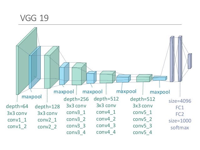\n\n","metadata":{"_uuid":"54c5c8da0c9d25d923ad94ceef7afd140dcfa97f"}},{"cell_type":"code","source":"import os\nimport random\nimport numpy as np\nimport matplotlib.pyplot as plt\nimport seaborn as sns\n\nfrom tensorflow.keras.preprocessing import image\nfrom tensorflow.keras.applications.vgg19 import VGG19, preprocess_input, decode_predictions\nfrom PIL import Image\n\n# Load VGG19 (pretrained on ImageNet)\n\nvgg19_model = VGG19(weights=\"imagenet\")\n\n# Folder containing test images\n\nfolder = \"/kaggle/input/cat-dog/test/test\"\n\n# Random sample of 5 images\n\nall_images = [os.path.join(folder, f) \n for f in os.listdir(folder) \n if f.lower().endswith((\".jpg\", \".png\", \".jpeg\"))]\n\nnum_sample = 5\nsample_images = random.sample(all_images, num_sample)\n\n# Run the plotter\n\nplot_predictions(vgg19_model, sample_images)\n","metadata":{"trusted":true,"_uuid":"73e61439cdc48836234deda711db6839ad975013","execution":{"iopub.status.busy":"2025-11-21T06:21:05.171747Z","iopub.execute_input":"2025-11-21T06:21:05.172028Z","iopub.status.idle":"2025-11-21T06:21:10.118696Z","shell.execute_reply.started":"2025-11-21T06:21:05.172009Z","shell.execute_reply":"2025-11-21T06:21:10.117903Z"}},"outputs":[],"execution_count":null},{"cell_type":"markdown","source":"## 1.3 InceptionNets\n\nAlso known as GoogleNet consists of total 22 layers and was the winning model of 2014 image net challenge. \n\n- Inception modules are the fundamental block of InceptionNets. The key idea of inception module is to design good local network topology (network within a network) \n- These modules or blocks acts as the multi-level feature extractor in which convolutions of different sizes are obtained to create a diversified feature map\n- The inception modules also consists of 1 x 1 convolution blocks whose role is to perform dimentionaltiy reduction. \n- By performing the 1x1 convolution, the inception block preserves the spatial dimentions but reduces the depth. So the overall network's dimentions are not increased exponentially. \n- Apart from the regular output layer, this network also consists of two auxillary classification outputs which are used to inject gradients at lower layers. \n\n
\n\nThe inception module is shown in the following figure: \n\n\n\n
\n\n### Pre-Trained Model : InceptionV3","metadata":{"_uuid":"864680ffb526762ccad64f0d6f95c886de12b2c3"}},{"cell_type":"code","source":"import os\nimport random\nimport numpy as np\nimport matplotlib.pyplot as plt\nimport seaborn as sns\n\nfrom tensorflow.keras.preprocessing import image\nfrom tensorflow.keras.applications.inception_v3 import InceptionV3, preprocess_input as inception_pre, decode_predictions as inception_decode\nfrom tensorflow.keras.applications.resnet50 import ResNet50, preprocess_input as resnet_pre, decode_predictions as resnet_decode\nfrom tensorflow.keras.applications.xception import Xception, preprocess_input as xception_pre, decode_predictions as xception_decode\n\nfrom PIL import Image\n\n\n# ---------------------------------------------------\n# Load all three pretrained models\n# ---------------------------------------------------\nmodel_inception = InceptionV3(weights=\"imagenet\")\nmodel_resnet = ResNet50(weights=\"imagenet\")\nmodel_xception = Xception(weights=\"imagenet\")\n\n\n# ---------------------------------------------------\n# Folder containing test images\n# ---------------------------------------------------\nfolder = \"/kaggle/input/cat-dog/test/test\"\n\n\n# ---------------------------------------------------\n# Random sample of 5 images\n# ---------------------------------------------------\nall_images = [os.path.join(folder, f)\n for f in os.listdir(folder)\n if f.lower().endswith((\".jpg\", \".jpeg\", \".png\"))]\n\nnum_sample = 5\nsample_images = random.sample(all_images, num_sample)\n\n\n# ---------------------------------------------------\n# Load + preprocess (generic, model-specific preprocess chosen later)\n# ---------------------------------------------------\ndef load_image(img_path, target_size):\n img = image.load_img(img_path, target_size=target_size)\n raw = img.copy()\n\n x = image.img_to_array(img)\n x = np.expand_dims(x, axis=0)\n return raw, x\n\n\n# ---------------------------------------------------\n# Generic prediction + plotting function\n# ---------------------------------------------------\ndef plot_predictions(model, model_name, preprocess_fn, decode_fn, img_paths, target_size):\n fig, axes = plt.subplots(2, len(img_paths), figsize=(6 * len(img_paths), 10))\n fig.suptitle(model_name + \" Predictions\", fontsize=20)\n\n for i, img_path in enumerate(img_paths):\n raw_img, x = load_image(img_path, target_size)\n x = preprocess_fn(x)\n\n preds = model.predict(x)\n top_preds = decode_fn(preds, top=3)[0]\n\n # Row 1: show image\n axes[0, i].imshow(raw_img)\n axes[0, i].set_title(\"Image\", fontsize=14)\n axes[0, i].axis(\"off\")\n\n # Row 2: bar plot\n sns.barplot(\n x=[p[2] for p in top_preds],\n y=[p[1] for p in top_preds],\n color=\"gray\",\n ax=axes[1, i]\n )\n axes[1, i].set_xlabel(\"Probability\")\n axes[1, i].set_title(os.path.basename(img_path))\n\n plt.tight_layout()\n plt.show()\n\n# InceptionV3 (input size: 299 × 299)\nplot_predictions(\n model_inception, \"InceptionV3\",\n inception_pre, inception_decode,\n sample_images, target_size=(299,299)\n)","metadata":{"trusted":true,"_uuid":"55f1b29e8180ddf39cf86886d2086566de21d0f4","execution":{"iopub.status.busy":"2025-11-21T06:55:29.610137Z","iopub.execute_input":"2025-11-21T06:55:29.610427Z","iopub.status.idle":"2025-11-21T06:55:41.611660Z","shell.execute_reply.started":"2025-11-21T06:55:29.610409Z","shell.execute_reply":"2025-11-21T06:55:41.610534Z"}},"outputs":[],"execution_count":null},{"cell_type":"markdown","source":"## 1.4 Resnets\n\nOriginal Paper : https://arxiv.org/pdf/1512.03385.pdf\n\nAll the previous models used deep neural networks in which they stacked many convolution layers one after the other. It was learnt that deeper networks are performing better. However, it turned out that this is not really true. Following are the problems with deeper networks: \n\n- Network becomes difficult to optimize \n- Vanishing / Exploding Gradeints \n- Degradation Problem ( accuracy first saturates and then degrades ) \n\n### Skip Connections \n\nSo to address these problems, authors of the resnet architecture came up with the idea of skip connections with the hypothesis that the deeper layers should be able to learn something as equal as shallower layers. A possible solution is copying the activations from shallower layers and setting additional layers to identity mapping. These connections are enabled by skip connections which are shown in the following figure. \n\n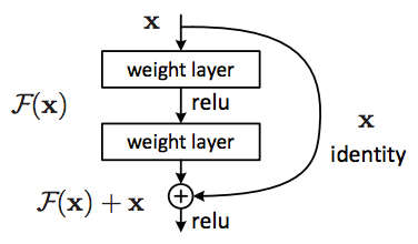\n\nSo the role of these connections is to perform identity function over the activation of shallower layer, which in-turn produces the same activation. This output is then added with the activation of the next layer. To enable these connections or essentially enable this addition operation, one need to ensure the same dimentions of convolutions through out the network, that's why resnets have same 3 by 3 convolutions throughout. \n\n### Key Advantage \n\nBy using residual blocks in the network, one can construct networks of any depth with the hypothesis that new layers are actually helping to learn new underlying patterns in the input data. The authors of the paper were able to create the deep neural network architecture with 152 layers. The variants of Resnets such as resnet34, resnet50, resnet101 have produced the solutions with very high accuracy in Imagenet competitions. \n\n### Why it works ? \n\nLets discuss why residual networks are successful and enables the addition of more and more layers without the key problems ie. without hurting the network performance. \n\nConsider a plain neural network (A) without residual network as shown. So in the network (A) the input X is passed to this Neural Network (NN) to give the activation A1. \n\n
\n\n\n\nNow, consider a more deeper network (B) in which a residual block (with 2 extra layers and a skip connection) is added in the previous network. So now, the activation A1 is being passed to Residual Block which in turns gives new activation A3. \n\nif there was no skip connection, then A3 was: \n\n> A3 = relu ( W2 . A2 + b2) ..... (without skip connection)\n\nwhere W2 and b2 are weights and bias associated with layer L2. But, with skip connection another term A1 will be passed to L2. So the equation of A3 will be modified as: \n\n> A3 = relu ( W2 . A2 + b2 + A1) \n\nIf we use L2 regularization or the weight decay methods, they will force W2 and b2 to become close to zero. In the worst case, if these become zero, then \n\n> A3 = relu (A1) \n\nbecause relu will output 0 for negative, A1 for positive and we know that A1 is previous activation from relu which is positive. \n\n> A3 = A1 \n\nThis means that Identitiy function is easy for residual blocks to learn. By addition of residual blocks, model complexity was not increased. As this is only copying the previous activation to the next layers. However this is only the worst case situation, but the it may turn out that these additional layers learns something useful. In that case, the network performance will improve. \n\nHence, adding the residual blocks / skip connections does not hurt the network performance but infact increases the chances that new layers will learn something useful. \n\nLet's look at the usage using pre-trained resnet 50 model. ","metadata":{"_uuid":"bfb5488e2aaf9f46d92aed89021fc4a3a27bbf19"}},{"cell_type":"code","source":"# ResNet50 (input size: 224 × 224)\nplot_predictions(\n model_resnet, \"ResNet50\",\n resnet_pre, resnet_decode,\n sample_images, target_size=(224,224)\n)","metadata":{"trusted":true,"_uuid":"7e8441e52f70fe3103312dc9e1dd0cd103e90e66","execution":{"iopub.status.busy":"2025-11-21T06:56:23.913206Z","iopub.execute_input":"2025-11-21T06:56:23.913490Z","iopub.status.idle":"2025-11-21T06:56:30.081508Z","shell.execute_reply.started":"2025-11-21T06:56:23.913472Z","shell.execute_reply":"2025-11-21T06:56:30.080547Z"}},"outputs":[],"execution_count":null},{"cell_type":"markdown","source":"## 1.5 Xception Nets\n\nXception is an extension of the Inception architecture which replaces the standard Inception modules with depthwise separable convolutions.","metadata":{"_uuid":"53c26efe9ea54cfc0852ebe389fb05592307d864"}},{"cell_type":"code","source":"# Xception (input size: 299 × 299)\nplot_predictions(\n model_xception, \"Xception\",\n xception_pre, xception_decode,\n sample_images, target_size=(299,299)\n)","metadata":{"trusted":true,"_uuid":"584f18cd3ce168413f72076362db2663e6442baf","execution":{"iopub.status.busy":"2025-11-21T06:56:47.152103Z","iopub.execute_input":"2025-11-21T06:56:47.152654Z","iopub.status.idle":"2025-11-21T06:56:52.633990Z","shell.execute_reply.started":"2025-11-21T06:56:47.152632Z","shell.execute_reply":"2025-11-21T06:56:52.632811Z"}},"outputs":[],"execution_count":null},{"cell_type":"markdown","source":"#### Comparison of different architectures: \n\nThe following image describes the relative comparison of these architectures in terms of performance as size. \n\n\n## 2. Image Feature Extraction using PreTrained Models \n\nLets look at how one can use pre-trained models for feature extraction, The extracted features can be used for Machine Learning purposes. \n\nFirst step is to load the weights of the pre-trained model in the model architecture. Notice, that an additional argument is passed include_top = False, which states that we do not want to add the last layer of this architecture. ","metadata":{"_uuid":"dadcad36efb34766ecb244797f6339e2ee14067f"}},{"cell_type":"code","source":"from tensorflow.keras.applications.resnet50 import ResNet50, preprocess_input\nfrom tensorflow.keras.preprocessing import image\nimport numpy as np\n\n# ---------------------------------------\n# Load pretrained ResNet50 WITHOUT top layer\n# ---------------------------------------\nresnet50 = ResNet50(weights=\"imagenet\", include_top=False)\n\n\n# ---------------------------------------\n# Function to extract deep features\n# ---------------------------------------\ndef get_features(img_path):\n img = image.load_img(img_path, target_size=(224, 224))\n img_data = image.img_to_array(img)\n img_data = np.expand_dims(img_data, axis=0)\n img_data = preprocess_input(img_data)\n\n # Extract convolutional feature maps\n features = resnet50.predict(img_data)\n\n return features\n\n\n# ---------------------------------------\n# Example: Extract features for 1 image\n# ---------------------------------------\nimg_path = \"/kaggle/input/cat-dog/test/test/10006.jpg\"\nresnet_features = get_features(img_path)\n\n# Two possible flattened representations\nfeatures_flat_1 = resnet_features.flatten()\nfeatures_flat_2 = resnet_features.squeeze()\n\n# Print shapes\nprint(\"Output Feature Map Shape (raw):\", resnet_features.shape)\nprint(\"Flatten using .flatten(): \", features_flat_1.shape)\nprint(\"Flatten using .squeeze(): \", features_flat_2.shape)\n","metadata":{"trusted":true,"_uuid":"eb48827bfad5ff9bfddbe9df991d32e3449f9451","execution":{"iopub.status.busy":"2025-11-21T06:59:17.030871Z","iopub.execute_input":"2025-11-21T06:59:17.031150Z","iopub.status.idle":"2025-11-21T06:59:23.090738Z","shell.execute_reply.started":"2025-11-21T06:59:17.031131Z","shell.execute_reply":"2025-11-21T06:59:23.090126Z"}},"outputs":[],"execution_count":null},{"cell_type":"markdown","source":"## 3. Transfer Learning Example \n\n
\n\nLets look at the implemetation of transfer learning using pre-trained model features. First, we 'll create a dataset containing two classes of images : bananas and strawberrys. Also add a test dataset contianing images from both classes.\n\n### 3.1 Dataset Preparation","metadata":{"_uuid":"145461de10bdd86deeaa1bfb27af0a4e5f8eaeff"}},{"cell_type":"code","source":"# import kagglehub\n\n# # Download latest version\n# path = kagglehub.dataset_download(\"moltean/fruits\")\n\n# print(\"Path to dataset files:\", path)","metadata":{"trusted":true,"execution":{"iopub.status.busy":"2025-11-21T07:08:36.079079Z","iopub.execute_input":"2025-11-21T07:08:36.080048Z","iopub.status.idle":"2025-11-21T07:08:37.683935Z","shell.execute_reply.started":"2025-11-21T07:08:36.080023Z","shell.execute_reply":"2025-11-21T07:08:37.683122Z"}},"outputs":[],"execution_count":null},{"cell_type":"code","source":"basepath = \"/kaggle/input/fruits/fruits-360_100x100/fruits-360/Training/\"\n\nclassA = \"Apple Crimson Snow 1\"\nclassB = \"Cherry 3\"\n\nfiles_A = os.listdir(os.path.join(basepath, classA))\nfiles_B = os.listdir(os.path.join(basepath, classB))\n\nprint(\"Samples in A:\", len(files_A))\nprint(\"Samples in B:\", len(files_B))","metadata":{"trusted":true,"_uuid":"d075c7be0c290ff513df855fe1707ea145ab9330","execution":{"iopub.status.busy":"2025-11-21T07:12:45.055543Z","iopub.execute_input":"2025-11-21T07:12:45.056412Z","iopub.status.idle":"2025-11-21T07:12:45.065706Z","shell.execute_reply.started":"2025-11-21T07:12:45.056387Z","shell.execute_reply":"2025-11-21T07:12:45.064895Z"}},"outputs":[],"execution_count":null},{"cell_type":"code","source":"resnet = ResNet50(weights=\"imagenet\", include_top=False)","metadata":{"trusted":true,"execution":{"iopub.status.busy":"2025-11-21T07:12:59.273311Z","iopub.execute_input":"2025-11-21T07:12:59.273887Z","iopub.status.idle":"2025-11-21T07:13:00.261110Z","shell.execute_reply.started":"2025-11-21T07:12:59.273863Z","shell.execute_reply":"2025-11-21T07:13:00.260558Z"}},"outputs":[],"execution_count":null},{"cell_type":"markdown","source":"Transfer learning can be implemented in two steps: \n\nStep 1 : Image Feature Exraction \nStep 2 : Training a Classifier \n\n### Step 1 : Feature Extraction using pre-trained models (resnet50)\n\nIterate in the images, call the same function used in point 2 for image feature extraction, we will use the flatten representation of these features ","metadata":{"_uuid":"5c3f81bf1bdf0266e09e180ef4fecd8c4e61cc8e"}},{"cell_type":"code","source":"def extract_features(img_path):\n img = image.load_img(img_path, target_size=(224,224))\n x = image.img_to_array(img)\n x = np.expand_dims(x, axis=0)\n x = preprocess_input(x)\n\n feat = resnet.predict(x) # Shape: (1, 7, 7, 2048)\n feat = feat.flatten() # Flatten to 100352 vector\n return feat","metadata":{"trusted":true,"_uuid":"715ae76b5aca0b8fce478fe1a3c2c9639c7bd789","execution":{"iopub.status.busy":"2025-11-21T07:13:14.052445Z","iopub.execute_input":"2025-11-21T07:13:14.053010Z","iopub.status.idle":"2025-11-21T07:13:14.056999Z","shell.execute_reply.started":"2025-11-21T07:13:14.052989Z","shell.execute_reply":"2025-11-21T07:13:14.056221Z"}},"outputs":[],"execution_count":null},{"cell_type":"markdown","source":"Next, Convert the features from dictionary format to pandas dataframe. A long dataframe will be created. I will be applying variance filter later on this dataframe to reduce the dimentionality. Other ideas to avoid this step : perform PCA / SVD to obtain the dense features. ","metadata":{"_uuid":"0fecb0e6eb0759b69ccf58cb255cc2f6751216b3"}},{"cell_type":"code","source":"X, y = [], []\n\ndef safe_extract(filepath):\n try:\n feat = extract_features(filepath)\n if feat is None or feat.shape[0] == 0:\n return None\n return feat\n except:\n return None\n\n\n# Class A = 0\nfor fname in files_A[:10]:\n fpath = os.path.join(basepath, classA, fname)\n feat = safe_extract(fpath)\n if feat is not None:\n X.append(feat)\n y.append(0)\n\n# Class B = 1\nfor fname in files_B[:10]:\n fpath = os.path.join(basepath, classB, fname)\n feat = safe_extract(fpath)\n if feat is not None:\n X.append(feat)\n y.append(1)\n\nX = np.array(X, dtype=np.float32)\ny = np.array(y)\n\nprint(\"X shape:\", X.shape) # expect (20, 100352)\nprint(\"y shape:\", y.shape) # expect (20,)\n","metadata":{"trusted":true,"scrolled":true,"_uuid":"57970a5ba3a19144849babd51102424a531cd207","execution":{"iopub.status.busy":"2025-11-21T07:15:14.726444Z","iopub.execute_input":"2025-11-21T07:15:14.726745Z","iopub.status.idle":"2025-11-21T07:15:16.432308Z","shell.execute_reply.started":"2025-11-21T07:15:14.726726Z","shell.execute_reply":"2025-11-21T07:15:16.431748Z"}},"outputs":[],"execution_count":null},{"cell_type":"markdown","source":"Prepare X (predictors) and y (target) from the dataset","metadata":{"_uuid":"254f97b6e4cecd5a8b8e4ee3ddf300a4d878968e"}},{"cell_type":"code","source":"y = to_categorical(y, 2)","metadata":{"trusted":true,"execution":{"iopub.status.busy":"2025-11-21T07:15:30.316381Z","iopub.execute_input":"2025-11-21T07:15:30.316670Z","iopub.status.idle":"2025-11-21T07:15:30.320374Z","shell.execute_reply.started":"2025-11-21T07:15:30.316651Z","shell.execute_reply":"2025-11-21T07:15:30.319627Z"}},"outputs":[],"execution_count":null},{"cell_type":"code","source":"from tensorflow.keras.utils import to_categorical\nfrom tensorflow.keras.models import Sequential\nfrom tensorflow.keras.layers import Dense, Dropout\n\nmodel = Sequential([\n Dense(256, activation='relu', input_shape=(X.shape[1],)),\n Dropout(0.3),\n Dense(128, activation='relu'),\n Dense(2, activation='softmax')\n])\n\nmodel.compile(optimizer='adam', loss='categorical_crossentropy', metrics=['accuracy'])\nmodel.summary()\n","metadata":{"trusted":true,"_uuid":"8732b6bd71eb01c4fc7bda6faf7d999d062aab76","execution":{"iopub.status.busy":"2025-11-21T07:15:49.495359Z","iopub.execute_input":"2025-11-21T07:15:49.495851Z","iopub.status.idle":"2025-11-21T07:15:49.538449Z","shell.execute_reply.started":"2025-11-21T07:15:49.495830Z","shell.execute_reply":"2025-11-21T07:15:49.537829Z"}},"outputs":[],"execution_count":null},{"cell_type":"code","source":"model.fit(X, y, epochs=10, batch_size=4, verbose=1)","metadata":{"trusted":true,"execution":{"iopub.status.busy":"2025-11-21T07:15:49.946748Z","iopub.execute_input":"2025-11-21T07:15:49.947200Z","iopub.status.idle":"2025-11-21T07:15:54.024921Z","shell.execute_reply.started":"2025-11-21T07:15:49.947181Z","shell.execute_reply":"2025-11-21T07:15:54.024302Z"}},"outputs":[],"execution_count":null},{"cell_type":"markdown","source":"### Step 2: Write a classifier to predict two classes\n\nwe will write a simple neural network (multi layer perceptron classifier) using sklearn for training purposes. ","metadata":{"_uuid":"d9af01bdf68adfce750b88fa13ff4cd85db580b4"}},{"cell_type":"code","source":"testA = os.path.join(basepath, classA, files_A[11])\ntestB = os.path.join(basepath, classB, files_B[11])\n\ntest_files = [testA, testB]\n\nclass_names = ['Apple Crimson Snow', 'Cherry']\n\nfor tf in test_files:\n feat = extract_features(tf)\n feat = np.expand_dims(feat, axis=0)\n\n pred = model.predict(feat)\n cls = np.argmax(pred)\n\n print(tf, \"→\", class_names[cls])\n","metadata":{"trusted":true,"_uuid":"feeefbaa75207a3c4bea5dc189b47dd7269224ff","execution":{"iopub.status.busy":"2025-11-21T07:15:56.378862Z","iopub.execute_input":"2025-11-21T07:15:56.379791Z","iopub.status.idle":"2025-11-21T07:15:57.268825Z","shell.execute_reply.started":"2025-11-21T07:15:56.379763Z","shell.execute_reply":"2025-11-21T07:15:57.268104Z"}},"outputs":[],"execution_count":null},{"cell_type":"markdown","source":"# **SUMMARY — FROM BEGINNING TO END (ALL STEPS)**\n\n---\n\n## ** PART 1 — Building VGG Networks & Running Predictions**\n\n### **1. Defined VGG16 architecture manually**\n\n* Constructed convolutional blocks (conv → conv → pool)\n* Added fully connected layers (4096 → 4096 → 1000 softmax)\n* Model input originally `(224,224,1)` → not suitable for ImageNet\n* Custom model had **random weights**, therefore predictions were meaningless\n\n### **2. Loaded pretrained VGG16**\n\n* Replaced manual model with:\n\n ```python\n vgg16_model = VGG16(weights='imagenet')\n ```\n* Pretrained VGG16 uses `(224,224,3)` images\n* Then predictions became correct\n\n### **3. Wrote prediction function**\n\n* Loaded images from disk\n* Preprocessed using `preprocess_input`\n* Used `decode_predictions` to get top-3 classes\n* Displayed images and prediction bar plots\n* Fixed subplot issues to show all images properly\n\n### **4. Identified GPU log messages**\n\n* GPU logs like “cuDNN loaded” were harmless\n* Used `os.environ['TF_CPP_MIN_LOG_LEVEL']='3'` to reduce logs\n* Fixed seaborn warnings with numpy arrays\n\n### **5. Plotted predictions for random test images**\n\n* Selected random images from cat-dog test folder\n* Corrected subplot layout\n* Displayed 5 images with top-3 predictions\n\n---\n\n## ** PART 2 — Using VGG19, Inception, ResNet50, Xception**\n\n### **6. Loaded multiple pretrained models**\n\n* VGG19\n* InceptionV3\n* ResNet50\n* Xception\n\nEach has different input sizes:\n\n* VGG / ResNet → 224×224\n* Inception / Xception → 299×299\n\n### **7. Created general-purpose prediction function**\n\n* Accepts model, preprocess method, decode function\n* Shows image + bar plot under each\n* Loops over `num_sample = 5` random images\n\n---\n\n## ** PART 3 — Feature Extraction with ResNet50**\n\n### **8. Loaded ResNet50 without classifier**\n\n```python\nresnet50 = ResNet50(weights='imagenet', include_top=False)\n```\n\n### **9. Built feature extraction function**\n\n* Loaded image to 224×224\n* Preprocessed\n* Predicted feature maps `(1,7,7,2048)`\n* Flattened to `(100352,)` feature vector\n\n### **10. Fixed shape & dtype issues**\n\n* Ensured all feature vectors have same shape\n* Removed invalid files with extension filtering\n* Converted X to `np.array(X, dtype=np.float32)`\n* Avoided inconsistent arrays that break Keras\n\n---\n\n## ** PART 4 — Transfer Learning (Two-Class Classification)**\n\n### **11. Identified your actual Kaggle dataset**\n\nYour Fruits-360_100x100 dataset contained classes like:\n\n* Apple Crimson Snow 1\n* Cherry 3\n* Pear\n* Onion\n* Tomato\n* Avocado\n (no Banana or Strawberry)\n\n### **12. Selected two valid classes**\n\nExample chosen:\n\n* **Apple Crimson Snow 1** → Label 0\n* **Cherry 3** → Label 1\n\n### **13. Extracted ResNet50 features**\n\n* Took 10 samples from each class\n* Extracted flattened feature vectors\n* Labeled them 0 or 1\n* One-hot encoded labels\n\n### **14. Built a simple classifier**\n\nUsing extracted features as input:\n\n```\nDense(256, relu)\nDropout(0.3)\nDense(128, relu)\nDense(2, softmax)\n```\n* Predicted class names correctly (Apple or Cherry)\n\n---\n\n### **15. Fixed \"Unrecognized data type\" error**\n\nCaused by:\n\n* invalid image files\n* inconsistent shapes\n* empty feature vectors\n\nSolution:\n\n* filter images by extension\n* check shapes before appending\n* convert `X` to valid numpy array","metadata":{}},{"cell_type":"code","source":"","metadata":{"trusted":true},"outputs":[],"execution_count":null}]}