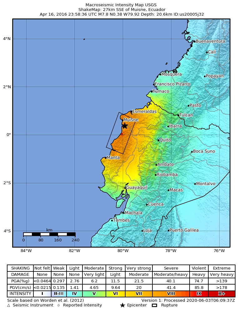
{"cells":[{"metadata":{},"cell_type":"markdown","source":"# Favorita Unit Sales Forecasting\n\nEDA and Machine Learning techniques applied with Python on Favorita Unit Sales to forecast future sales.\n\n\n# Table of Contents\n* Business Understanding\n* Data Understainding\n* Data Preparation\n* Modelling\n* Evaluation\n* Deployment\n* Credits\n\n\n# Business Understanding\nBrick-and-mortar grocery stores are always in a delicate dance with purchasing and sales forecasting. Predict a little over, and grocers are stuck with overstocked, perishable goods. Guess a little under, and popular items quickly sell out, leaving money on the table and customers fuming.\n\nThe problem becomes more complex as retailers add new locations with unique needs, new products, ever transitioning seasonal tastes, and unpredictable product marketing. Corporación Favorita, a large Ecuadorian-based grocery retailer, knows this all too well. They operate hundreds of supermarkets, with over 200,000 different products on their shelves.\n\nCorporación Favorita has [challenged the Kaggle community](https://www.kaggle.com/c/favorita-grocery-sales-forecasting) to build a model that more accurately forecasts product sales. They currently rely on subjective forecasting methods with very little data to back them up and very little automation to execute plans. They’re excited to see how machine learning could better ensure they please customers by having just enough of the right products at the right time.\n\nFrom the result of the predictions we will draw few solutions and recommendations on how to maximize the future earnings of Favorita stores.\n\n**⚠ IMPORTANT NOTES**\n* Wages in the public sector are paid every two weeks on the 15th and on the last day of the month. Supermarket sales could be affected by this.\n* A magnitude 7.8 earthquake struck Ecuador on April, the 16th 2016 at 18:58 ECT. People rallied in relief efforts donating water and other first need products which greatly affected supermarket sales for several weeks after the earthquake. For more info about the earthquake, see [Wikipedia](https://en.wikipedia.org/wiki/2016_Ecuador_earthquake).
 "},{"metadata":{"trusted":true,"_kg_hide-output":true,"collapsed":true},"cell_type":"code","source":"# install third-party dependencies\n!python -m pip install --upgrade pip\n!pip install py7zr\n!pip install seaborn --upgrade\n# interpreter version\n!python --version","execution_count":null,"outputs":[]},{"metadata":{"trusted":true},"cell_type":"code","source":"# data processing\nimport py7zr\nimport os\nimport datetime\nimport numpy as np\nimport pandas as pd\n# visualization\nimport matplotlib.pyplot as plt\nimport seaborn as sns\nimport plotly.graph_objects as go\nimport plotly.express as px","execution_count":null,"outputs":[]},{"metadata":{"trusted":true},"cell_type":"code","source":"# helper functions\n\ndef add_axis_vline(ax, x, y, text):\n \"\"\"\n Add vertical line to timeseries plot.\n \"\"\"\n ax.axvline(x=x, ymin=0, ymax=y, c='r', ls=':')\n ax.text(x=x, y=y, s=text, verticalalignment='top', rotation=270)\n\n\ndef missing_dates(dates):\n \"\"\"\n Find missing dates from a passed Pandas DataFrame.\n Expected date column name= `date`\n Return the original data if dates are no missing\n \"\"\"\n actual = dates.unique()\n total = pd.date_range(dates.min(), dates.max())\n missing = pd.DataFrame({'date': total ^ pd.Index(actual)})\n assert len(total) - len(actual) == len(missing), f'# total ({len(total)}) - # actual ({len(actual)}) != # missing dates ({len(missing)})'\n print(len(missing), 'missing dates found')\n return missing\n\n\ndef data_model(data, feature_id):\n \"\"\"\n Create data model as M*N matrix of features where\n M are the samples (store_id & item_id to identify each data point),\n N are the features (date of the timeline).\n The Mi*Ni is the feature value.\n \"\"\"\n tmp_data = data.copy() # do NOT change the input data for future computations\n return tmp_data.pivot(index=['store_nbr', 'item_nbr'], columns='date', values=feature_id)\n\n\n# create an interactive visualization tool to analyze each product individually to search\n# for any potential relation with the features available agains the target (i.e. unit_sales).\ndef plot_unit_sales(item_nbr, store_nbr):\n \"\"\"\n Interactive plot to allow fast EDA of specific features\n \"\"\"\n # item/store info\n item_info = items.set_index('item_nbr').loc[item_nbr]\n store_info = stores.set_index('store_nbr').loc[store_nbr]\n # chart title\n title = f\"#{item_nbr} item unit sales\\n{', '.join([f'{k}={v}' for k,v in item_info.items()])}\\n{', '.join([f'{k}={v}' for k,v in store_info.items()])}\"\n print(title)\n # select data\n tmp_item = df_train[(df_train['store_nbr'] == store_nbr) & (df_train['item_nbr'] == item_nbr)]\n tmp_item.drop(columns=['store_nbr', 'item_nbr'], inplace=True)\n tmp_item.sort_values('date', inplace=True)\n # boolean holiday (local and regional are grouped together)\n national_holidays = holidays['locale'] == 'National'\n tmp_item['is_holiday'] = tmp_item['date'].isin(holidays['date'][national_holidays])\n # merge oil\n tmp_item = tmp_item.merge(oil, on='date')\n # dates (x-axis) and sales (y-axis)\n dates = tmp_item['date']\n sales = tmp_item['unit_sales']\n # items on promotion\n promo = tmp_item['onpromotion'] == True\n promo_dates = dates[promo]\n promo_unit_sales = sales[promo]\n # scale and smoot values\n oil_scaler = MinMaxScaler(feature_range=(sales.min(), sales.max()))\n scaled_oil = oil_scaler.fit_transform(tmp_item['dcoilwtico'].values.reshape(-1, 1)).flatten()\n sales_smooth = sales.ewm(span=len(tmp_item)*.1).mean()\n # figure\n fig = go.Figure([\n go.Scatter(\n name='promo',\n x=promo_dates,\n y=promo_unit_sales,\n mode='markers',\n marker=dict(color='red', size=5),\n showlegend=True\n ),\n go.Scatter(\n name='unit sales',\n x=dates,\n y=sales,\n mode='lines',\n line=dict(color='black', width=.5),\n showlegend=True\n ),\n go.Scatter(\n name='moving avg',\n x=dates,\n y=sales_smooth,\n mode='lines',\n line=dict(color='royalblue', width=2, dash='dot'),\n showlegend=True\n ),\n go.Scatter(\n name='dcoilwtico',\n x=dates,\n y=scaled_oil,\n mode='lines',\n line=dict(color='coral', width=1),\n showlegend=True\n )\n ])\n fig.update_layout(\n title=title\n )\n fig.layout.template = 'plotly_white'\n return fig","execution_count":null,"outputs":[]},{"metadata":{},"cell_type":"markdown","source":"# Data Understanding\nIt is a regression problem applied on time series data. The main files are `train.csv` and `test.csv` and contain the daily items sales by store. The table below contains metadata for each dataset:\n\n*Table 1. Metadata*\n \n|Filename|Description|Notes|\n|--------|:----------|:----|\n|**`train.csv`**
**`test.csv`**|It contains the daily items sales by store for training and testing purposes|The followings apply to the datasets:
- the target `unit_sales` can be integer (e.g., a bag of chips) or float (e.g., 1.5 kg of cheese)
- there are a small number of items seen in the training data that aren't seen in the test data
- the training data does not include rows for items that had zero `unit_sales` for a store/date combination. There is no information as to whether or not the item was in stock for the store on the date, we will need to decide the best way to handle that situation
- approximately 16% of the `onpromotion` values are missing
- some test items are not included in the train data.
|\n|**`items.csv`**|Item metadata, including family, class, and perishable|- Items marked as perishable have a score weight of 1.25; otherwise, the weight is 1.0. This status will have a notable impact on our prediction models, because good predictions of perishable items are (understandably) rewarded with a bonus
- Missing metadata for parameter `class`.
|\n|**`stores.csv`**|Details about the stores, such as location and type||\n|**`oil.csv`**|Daily oil price includes values during both the train and test data timeframe|Ecuador is an oil-dependent country and it's economical health is highly vulnerable to shocks in oil prices|\n|**`holidays_events.csv`**|Holidays in Ecuador|- Pay special attention to the `transferred` column as holidays can be transferred to another day
- A `transferred` day is more like a normal day than a holiday
- Days that are type `Bridge` ares extra days that are added to a holiday. These are frequently made up by the type `Work Day` which is a day not normally scheduled for work (e.g., Saturday) that is meant to payback the `Bridge`
- `Additional` holidays are days added a regular calendar holiday.
|\n|**`transactions.csv`**|Count of sales transactions for the training data|This is only available for the training data.|"},{"metadata":{"trusted":true,"_kg_hide-input":true},"cell_type":"code","source":"%%time\n# in/output paths\ninput_path = '/kaggle/input/favorita-grocery-sales-forecasting'\noutput_path = '/kaggle/temp'\n# extract CSV files\nfiles = ['train', 'test', 'items', 'stores', 'holidays_events', 'oil', 'transactions']\nif not os.path.exists(output_path):\n for file in files:\n file_path = os.path.join(input_path, file+'.csv.7z')\n with py7zr.SevenZipFile(file_path, mode='r') as zipfile:\n zipfile.extractall(path=output_path)\n print('extracted:', file_path)\n\n# read CSV files\nprint('read train.csv')\ntrain = pd.read_csv(\n os.path.join(output_path, 'train.csv'),\n usecols=[1, 2, 3, 4, 5], # removing id column (index 0)\n dtype={'item_nbr': 'category', 'store_nbr': 'category', 'onpromotion': bool},\n parse_dates=['date'],\n skiprows=range(1, 101688779) # read from 2017-01-01 \n)\n\nprint('read test.csv')\ntest = pd.read_csv(\n os.path.join(output_path, 'test.csv'),\n dtype={'item_nbr': 'category', 'store_nbr': 'category', 'onpromotion': bool},\n parse_dates=['date']\n)\n\nprint('read items.csv')\nitems = pd.read_csv(\n os.path.join(output_path, 'items.csv'),\n dtype={'item_nbr': 'category', 'class': 'category', 'perishable': bool},\n)\n\nprint('read stores.csv')\nstores = pd.read_csv(\n os.path.join(output_path, 'stores.csv'),\n dtype={'store_nbr': 'category', 'city': 'category', 'state': 'category', 'type': 'category', 'cluster': 'category'},\n)\n\nprint('read holidays_events.csv')\nholidays = pd.read_csv(\n os.path.join(output_path, 'holidays_events.csv'),\n parse_dates=['date'],\n dtype={'type': 'category', 'local': 'category', 'locale_name': 'category'},\n skiprows=range(1, 42) # take holidays from 2013-01-01\n)\n\nprint('read oil.csv')\noil = pd.read_csv(\n os.path.join(output_path, 'oil.csv'),\n parse_dates=['date']\n)\n\nprint('read transactions.csv')\ntransactions = pd.read_csv(\n os.path.join(output_path, 'transactions.csv'),\n dtype={'store_nbr': 'category'},\n parse_dates=['date']\n)","execution_count":null,"outputs":[]},{"metadata":{},"cell_type":"markdown","source":"* all datasets take ~10gb of RAM\n* training set has 125.497.040 entries and the testing set has 3.370.464 entries\n* **Note that we selected a sub-sample between `2017-01-01` and `2017-08-15` to ease the computation and speed up the analysis**"},{"metadata":{},"cell_type":"markdown","source":"## Train"},{"metadata":{"trusted":true},"cell_type":"code","source":"train.head()","execution_count":null,"outputs":[]},{"metadata":{"trusted":true},"cell_type":"code","source":"train.info()","execution_count":null,"outputs":[]},{"metadata":{},"cell_type":"markdown","source":"* \\~450 mb of memory usage might become tricky with complex computations\n* `date` must be converted into or used to feature engineer number types\n* `onpromotion` sounds like an important features\n* Pandas `float64` types might contain missing values"},{"metadata":{"trusted":true},"cell_type":"code","source":"train.nunique()","execution_count":null,"outputs":[]},{"metadata":{},"cell_type":"markdown","source":"* `item_nbr` categorical feature has high cardinality"},{"metadata":{"trusted":true},"cell_type":"code","source":"train.describe()","execution_count":null,"outputs":[]},{"metadata":{},"cell_type":"markdown","source":"* `unit sales` is the target feature\n* no missing values are present\n* large range with min and max values between 1e-4 and 1e+4, respectively\n* \\~75% of unit sales are small values below 8.0 unit sales per item\n* there are negative unit sales (returned items) that represents a small portion of the sample"},{"metadata":{"trusted":true,"_kg_hide-input":true},"cell_type":"code","source":"fig, [[ax1, ax2], [ax3, ax4]] = plt.subplots(2, 2, figsize=(16, 8))\n# unit_sales (target)\nax1.set_title('Unit Sales distribution')\nax1.set_yscale('log') # normalize y\nax1.set_ylabel('frequency')\nax1.set_xlabel('unit sales (positive)')\nax1.hist(train.loc[train['unit_sales'] > 0., 'unit_sales'].transform(np.log))\n# date (daily data points count)\nax2.set_title('Count of Daily Unit Sales')\nax2.set_ylabel('daily count')\nax2.set_xlabel('dates')\ntrain['date'].value_counts().sort_index().plot.line(ax=ax2)\n# onpromotion \nax3.set_title('Onpromotion vs regular price')\nax3.set_ylabel('count %')\nax3.set_xlabel('onpromotion')\ntrain['onpromotion'].value_counts(normalize=True).plot.bar(ax=ax3)\n# store_nbr\nax4.set_title('Number of occurrences by store')\nax4.set_ylabel('count %')\nax4.set_xlabel('stores')\ntrain['store_nbr'].value_counts(normalize=True).plot.bar(ax=ax4)\nplt.tight_layout();","execution_count":null,"outputs":[]},{"metadata":{},"cell_type":"markdown","source":"* `unit_sales` follows the normal distribution (i.e. after log transformation of of values and frequency)\n* the number of data points by `date` collected seems stable but this is true for the sub-sample\n* vast majority of items are not `onpromotion`\n* 54 unique `store_nbr` are found in the sample\n * `store_nbr` whose number starts with `4` own majority of the data points"},{"metadata":{"trusted":true},"cell_type":"code","source":"missing_date_train = missing_dates(train['date'])","execution_count":null,"outputs":[]},{"metadata":{},"cell_type":"markdown","source":"## Test"},{"metadata":{"trusted":true},"cell_type":"code","source":"test.head()","execution_count":null,"outputs":[]},{"metadata":{"trusted":true},"cell_type":"code","source":"test.info()","execution_count":null,"outputs":[]},{"metadata":{"trusted":true},"cell_type":"code","source":"test.nunique()","execution_count":null,"outputs":[]},{"metadata":{},"cell_type":"markdown","source":"* there are 99 items missing from the test set as mentioned before; we need to decide to keep or remove them during training"},{"metadata":{"_kg_hide-input":true,"trusted":true},"cell_type":"code","source":"fig, [[ax1, ax2], [ax3, _]] = plt.subplots(2, 2, figsize=(16, 8))\n# date (daily data points count)\nax1.set_title('Count of Daily Unit Sales')\nax1.set_ylabel('daily count')\nax1.set_xlabel('dates')\ntest['date'].value_counts().sort_index().plot.line(ax=ax1)\n# onpromotion \nax2.set_title('Onpromotion vs regular price')\nax2.set_ylabel('count %')\nax2.set_xlabel('onpromotion')\ntest['onpromotion'].value_counts(normalize=True).plot.bar(ax=ax2)\n# store_nbr\nax3.set_title('Number of occurrences by store')\nax3.set_ylabel('count %')\nax3.set_xlabel('stores')\ntest['store_nbr'].value_counts(normalize=True).plot.bar(ax=ax3)\nplt.tight_layout()\n_.set_visible(False);","execution_count":null,"outputs":[]},{"metadata":{},"cell_type":"markdown","source":"* `unit_sales` is not present as we need to predict it\n* the number of data points by `date` collected is constant\n* `onpromotion` distribution on test set is similar to the one in the training set\n* `store_nbr` has a constant number of data points"},{"metadata":{"trusted":true},"cell_type":"code","source":"missing_date_test = missing_dates(test['date'])","execution_count":null,"outputs":[]},{"metadata":{},"cell_type":"markdown","source":"## Items"},{"metadata":{"trusted":true},"cell_type":"code","source":"items.describe()","execution_count":null,"outputs":[]},{"metadata":{},"cell_type":"markdown","source":"* all categorical (nominal) features\n* there are `4100` distinct items divided into `337` classes and `33` families\n* `GROCERY I` is the most popular family\n* `perishable` is very important boolean feature because `perishable` items have a score weight of 1.25 (otherwise, the weight is 1.0) in this competition; our model should be aware of it and be very reliable on their prediction (good predictions of perishable items are rewarded with a bonus)."},{"metadata":{"trusted":true,"_kg_hide-input":true},"cell_type":"code","source":"fig, [ax1, ax2] = plt.subplots(1, 2, figsize=(12,6))\n# perishable\nax1.set_title('Perishable vs non-perishable')\nax1.set_ylabel('count %')\nax1.set_xlabel('perishable')\nitems['perishable'].value_counts(normalize=True).plot.bar(ax=ax1)\n# family\nax2.set_title('Item count by family')\nax2.set_ylabel('count %')\nax2.set_xlabel('family')\nitems['family'].value_counts(normalize=True).plot.bar(ax=ax2)\nplt.tight_layout();","execution_count":null,"outputs":[]},{"metadata":{"trusted":true},"cell_type":"code","source":"# number of distinct families is equal to the number of distinct first-two-digit classes\nitems['class'].str[:2].nunique() == items['family'].nunique()","execution_count":null,"outputs":[]},{"metadata":{},"cell_type":"markdown","source":"* ~25% of items are of type `perishable`\n* top 3 families, `GROCERY I` (\\~33%), `BEVERAGES` (\\~15%), and `CLEANING` (~11%) are non-perishable items\n* given their frequencies, `GROCERY I` and `BEVERAGES` could be essential goods\n* `family` and `class` features abstract the structure of supermarkets: products (class) are organized into aisles (family)\n * in fact the first 2 digits of `class` refers to the `family` (e.g. class items starting with 10 are `GROCERY I`)"},{"metadata":{},"cell_type":"markdown","source":"## Stores"},{"metadata":{"trusted":true},"cell_type":"code","source":"stores.describe()","execution_count":null,"outputs":[]},{"metadata":{},"cell_type":"markdown","source":"* `54` distinct stores in `22` cities and `16` states\n* type `D` is the most popular among the 5 distinct types\n* majority of stores are in cluster `3`\n* not surprisingly, the capital `Quito` in the state of `Pichincha` is the place with most stores"},{"metadata":{"trusted":true,"_kg_hide-input":true},"cell_type":"code","source":"fig, [[ax1, ax2], [ax3, ax4]] = plt.subplots(2, 2, figsize=(12,6))\n# city\nax1.set_title('Number of stores by city')\nax1.set_xlabel('city')\nax1.set_ylabel('count')\nstores['city'].value_counts().plot.bar(ax=ax1)\n# state\nax2.set_title('Number of stores by state')\nax2.set_xlabel('state')\nax2.set_ylabel('count')\nstores['state'].value_counts().plot.bar(ax=ax2)\n# type\nax3.set_title('Number of stores by type')\nax3.set_xlabel('type')\nax3.set_ylabel('count')\nstores['type'].value_counts().plot.bar(ax=ax3)\n# cluster\nax4.set_title('Number of stores by cluster')\nax4.set_xlabel('cluster')\nax4.set_ylabel('count')\nstores['cluster'].value_counts().plot.bar(ax=ax4)\nplt.tight_layout();","execution_count":null,"outputs":[]},{"metadata":{},"cell_type":"markdown","source":"* the distributions of stores by `city` and by `state` show a similar trend\n* we can divided the stores counts by `city` and `state` in 4 distinct distributions\n* as expected most of the stores are located in the main cities `Quito` (\\~35%) and `Guayaquil` (\\~15%) (first distribution group)\n* there are 5 types of store but we do not have a clear understanding what kind of store each type represents\n* `type=D` is the most popular, perhaps the type is related to a particular sub-brand or size of supermarket under the [Corporacion Favorita](https://www.corporacionfavorita.com/marcas/area-comercial/) umbrella\n* it groups similar stores from different locations so we can deduct that unit sales of stores of same type are comparable even if the stores are in different locations\n* `5`, `12`, `16`, and `17` clusters have only one store (not much of a cluster)"},{"metadata":{"trusted":true},"cell_type":"code","source":"px.bar(stores.value_counts(subset=['state', 'city']).reset_index(name='stores'),\n x='state', y='stores', color='city', title='Number of stores by city and state')","execution_count":null,"outputs":[]},{"metadata":{},"cell_type":"markdown","source":"* most states have stores in just one city\n* `Los Rios` and `Pichincha` have 2 cities, `Guayas` has 4"},{"metadata":{},"cell_type":"markdown","source":"## Holidays Events"},{"metadata":{"trusted":true},"cell_type":"code","source":"holidays.describe()","execution_count":null,"outputs":[]},{"metadata":{"trusted":true,"_kg_hide-input":true},"cell_type":"code","source":"fig, [ax1, ax2, ax3, ax4] = plt.subplots(1, 4, figsize=(20,4))\n# type\nax1.set_title('Number of holidays by type')\nax1.set_ylabel('count')\nholidays['type'].value_counts().plot.bar(ax=ax1)\n# locale\nax2.set_title('Number of holidays by locale')\nax2.set_ylabel('count')\nholidays['locale'].value_counts().plot.bar(ax=ax2)\n# locale_name\nax3.set_title('Number of holidays by locale_name')\nax3.set_ylabel('count')\nholidays['locale_name'].value_counts().plot.bar(ax=ax3)\n# transferred\nax4.set_title('Number of holidays transferred')\nax4.set_ylabel('count')\nholidays['transferred'].value_counts().plot.bar(ax=ax4)\n# description\nfig, ax = plt.subplots(figsize=(20, 7))\nax.set_title('Number of holidays by description')\nax.set_xlabel('descriptions')\nax.set_ylabel('count')\nholidays['description'].value_counts().plot.bar(ax=ax)\nplt.tight_layout();","execution_count":null,"outputs":[]},{"metadata":{},"cell_type":"markdown","source":"* most of holidays are `national` or `local` types there are also ~10% `regional` holidays\n* it breaks down the information in `locale` (e.g. `equador`==`national`)\n* `carnaval` seems to be the most popular holiday\n* there is a large number of distinct descriptions that belong to mainly 2 groups:\n * 2014: `Terremoto-manabi-#`\n * 2016: `Mundial de futbol`\n* there is only a small % of transferred holidays which substitutes holidays of type `Transfer`"},{"metadata":{"trusted":true},"cell_type":"code","source":"# holidays by year and month\nyear = holidays['date'].dt.year.astype('category')\nyear.name = 'years'\nmonth = holidays['date'].dt.month.astype('category')\nmonth.name = 'months'\npx.imshow(\n holidays.value_counts([year, month]).sort_index().reset_index(name='holidays').pivot_table(\n index='years', columns='months', values='holidays', aggfunc='sum', fill_value=0\n ),\n x=['Jan', 'Feb', 'Mar', 'Apr', 'May', 'Jun', 'Jul', 'Aug', 'Sep', 'Oct', 'Nov', 'Dec'],\n labels=dict(color=\"# holidays\"), title='Year vs Month Holidays'\n)","execution_count":null,"outputs":[]},{"metadata":{"trusted":true},"cell_type":"code","source":"# remove transferred dates from holidays as considered regular days\nholidays = holidays[holidays['transferred'] == False]","execution_count":null,"outputs":[]},{"metadata":{},"cell_type":"markdown","source":"* In general, November and Dicember are the months with most holidays\n* January-March, September, and October are the months with less holidays, September with the least in absolute\n* 2014 Football World Cup (June-July) and 2016 earthquake (April-May) special holidays clearly stand out\n * many special holidays were introduced in May due to the earthquake\n* February 2014 has no holidays"},{"metadata":{},"cell_type":"markdown","source":"## Oil"},{"metadata":{"trusted":true},"cell_type":"code","source":"oil.describe()","execution_count":null,"outputs":[]},{"metadata":{"trusted":true},"cell_type":"code","source":"fig, [ax1, ax2] = plt.subplots(2, 1, figsize=(15, 12))\n# ewa (smoothing) factor (span)\nspan = len(oil)*.05\n# dcoilwtico\nax1.set_title('Daily oil price (dcoilwtico)')\nax1.set_xlabel('dates')\nax1.set_ylabel('dcoilwtico')\noil['dcoilwtico'].plot.line(ax=ax1, legend=True)\noil['dcoilwtico'].ewm(span=span).mean().plot.line(ax=ax1, style='r-', label='ewa', legend=True)\n# dcoilwtico 7-day price variation\nax2.set_title('7-day oil price (dcoilwtico) variation')\nax2.set_xlabel('dates')\nax2.set_ylabel('dcoilwtico variation')\nweekly_var = oil['dcoilwtico'] - oil['dcoilwtico'].shift(periods=7)\nweekly_var.plot.line(ax=ax2, legend=True)\nweekly_var.ewm(span=span).mean().plot.line(ax=ax2, style='r-', label='ewa', legend=True)\nplt.tight_layout();","execution_count":null,"outputs":[]},{"metadata":{},"cell_type":"markdown","source":"* note that oil data has missing values and dates so we need to add missing date and interpolate their oil price\n* we see a long-term change with an oil price dropped by half in the end of 2015\n* we observe large (7-day) variations between Q3 2014 and Q3 2015"},{"metadata":{"trusted":true},"cell_type":"code","source":"missing_dates_oil = missing_dates(oil['date'])\nmissing_dates_oil['dcoilwtico'] = None\noil_clean = pd.concat([oil, missing_dates_oil]).set_index('date').sort_index()\n# fix oil dataset\nif oil_clean['dcoilwtico'].isna().sum() > 0:\n oil_clean['dcoilwtico'].interpolate(method='linear', axis=0, limit=5, inplace=True)\n# check cleaned oil\nmissing_dates_oil = missing_dates(oil_clean.index)","execution_count":null,"outputs":[]},{"metadata":{},"cell_type":"markdown","source":"## Transactions"},{"metadata":{"trusted":true},"cell_type":"code","source":"transactions.describe()","execution_count":null,"outputs":[]},{"metadata":{"trusted":true},"cell_type":"code","source":"fig, ax = plt.subplots(figsize=(15, 6))\n# transactions\nax.set_title('Cumulative number of daily transactions')\nax.set_xlabel('dates')\nax.set_ylabel('transactions (median)')\ndaily_transactions = transactions.groupby('date')['transactions'].agg('median').reset_index()\ndaily_transactions['ewa'] = daily_transactions['transactions'].ewm(span=1682*.2).mean()\ndaily_transactions.set_index('date', inplace=True)\ndaily_transactions['transactions'].plot.line(ax=ax)\ndaily_transactions['ewa'].plot.line(ax=ax, style='r-')\n# earthquake 2016 mark\nadd_axis_vline(ax, x=np.datetime64('2016-04-16'), y=daily_transactions['transactions'].max(), text='earthquake');","execution_count":null,"outputs":[]},{"metadata":{"trusted":true},"cell_type":"code","source":"# number of days = 1682\n# double-click on a legend items to select it\npx.line(\n transactions.pivot_table(index='date', columns='store_nbr', values='transactions', aggfunc='median').ewm(span=1682*.2).mean(),\n title='Daily transactions count by store (exponential weighted average)'\n)","execution_count":null,"outputs":[]},{"metadata":{},"cell_type":"markdown","source":"* `transactions` are NOT available for the period of the test set (`2017-08-15 >`)\n* cumulative median number of daily transactions consistently show peak during Christmas and a drop on New Years Day, most likely due to the holidays\n* there is a jump in transactions numbers that coincides with the earthquake date (red)\n* as we saw before, store `52` had fewer data points then most of the stores because of its recent opening date\n* beside store `52`, the following stores opened after `2013-01-01`: `20`, `21`, `22`, `29`, `42`, `53`\n* we can better see the effects of the 2016 earthquake with a solid jump in the weighted average transactions of store `53"},{"metadata":{"trusted":true},"cell_type":"code","source":"# transactions distribution by store type\npx.box(\n transactions.merge(stores, on='store_nbr'), x='store_nbr', y='transactions',\n color='type', title='Transactions distribution by store type'\n).update_xaxes(categoryorder='median descending')","execution_count":null,"outputs":[]},{"metadata":{},"cell_type":"markdown","source":"* according to the transactions counts, type `A` stores show a consistenly higher distribution than any other store type\n* type `A` includes `store_nbr` from `44-52`\n* type `A` stores could either be maxi stores with a generally larger customers or wholesale stores with an higher minimum unit sales purchaseable"},{"metadata":{"trusted":true},"cell_type":"code","source":"missing_dates_transactions = missing_dates(transactions['date'])","execution_count":null,"outputs":[]},{"metadata":{},"cell_type":"markdown","source":"## Unit Sales Relations\n\nIn summary, the goal of this time-series forecasting problem is to predict the `unit_sales` (i.e. the target value) of a given item in the future.\n\nWe have a large number of training data points each of which is a distinct item sold by a certain store on a specific date. For each training data point we know the target value `unit_sales`. A Machine Learning model will be trained onto the training data points to predict the unknown target value `unit_sales` of the test data points.\n\nWe utilise the relations between the various time series features (e.g. type of item, location of store, day of the week) to improve our `unit_sales` predictions.\n\nFirst, we will isolate the `unit_sales` of few specific items and stores to have a better understanding of the data we are working with and that we need to predict. Thereafter, we will investigate the relations that the features share with out target value (`unit_sales`)."},{"metadata":{},"cell_type":"markdown","source":"## Most Popular Item and Store"},{"metadata":{"trusted":true},"cell_type":"code","source":"# most sold items\ntrain.groupby(by=['item_nbr', 'store_nbr'])['unit_sales'].sum().sort_values(ascending=False).to_frame().head(5)","execution_count":null,"outputs":[]},{"metadata":{"trusted":true},"cell_type":"code","source":"#plot_unit_sales(item_nbr='1503844', store_nbr='44')\n# item/store info\nitem_info = items.set_index('item_nbr').loc[item_nbr]\nstore_info = stores.set_index('store_nbr').loc[store_nbr]\n# chart title\ntitle = f\"#{item_nbr} item unit sales\\n{', '.join([f'{k}={v}' for k,v in item_info.items()])}\\n{', '.join([f'{k}={v}' for k,v in store_info.items()])}\"\nprint(title)\n# select data\ntmp_item = df_train[(df_train['store_nbr'] == store_nbr) & (df_train['item_nbr'] == item_nbr)].drop(columns=['store_nbr', 'item_nbr'])\ntmp_item.sort_values('date', inplace=True)\n# boolean holiday (local and regional are grouped together)\nnational_holidays = holidays['locale'] == 'National'\ntmp_item['is_holiday'] = tmp_item['date'].isin(holidays['date'][national_holidays])\n# merge oil\ntmp_item = tmp_item.merge(oil, on='date')\n# dates (x-axis) and sales (y-axis)\ndates = tmp_item['date']\nsales = tmp_item['unit_sales']\n# items on promotion\npromo = tmp_item['onpromotion'] == True\npromo_dates = dates[promo]\npromo_unit_sales = sales[promo]\n# scale and smooth values\noil_scaler = MinMaxScaler(feature_range=(sales.min(), sales.max()))\nscaled_oil = oil_scaler.fit_transform(tmp_item['dcoilwtico'].values.reshape(-1, 1)).flatten()\nsales_smooth = sales.ewm(span=len(tmp_item)*.1).mean()\n# figure\nfig = go.Figure([\n go.Scatter(\n name='promo',\n x=promo_dates,\n y=promo_unit_sales,\n mode='markers',\n marker=dict(color='red', size=5),\n showlegend=True\n ),\n go.Scatter(\n name='unit sales',\n x=dates,\n y=sales,\n mode='lines',\n line=dict(color='black', width=.5),\n showlegend=True\n ),\n go.Scatter(\n name='moving avg',\n x=dates,\n y=sales_smooth,\n mode='lines',\n line=dict(color='royalblue', width=2, dash='dot'),\n showlegend=True\n ),\n go.Scatter(\n name='dcoilwtico',\n x=dates,\n y=scaled_oil,\n mode='lines',\n line=dict(color='coral', width=1),\n showlegend=True\n )\n])\nfig.update_layout(\n title=title\n)\nfig.layout.template = 'plotly_white'\nfig.show()","execution_count":null,"outputs":[]},{"metadata":{},"cell_type":"markdown","source":"## Verifications\n\nLet's confirm the hints given in the competition intro: **Public Wages Incidence** and **2016 Earthquake**\n\n### Public Wages Incidence\n\nIn Ecuador, wages in the public sector are paid every two weeks on the 15th and on the last day of the month. **Supermarket sales could be affected by this**. We could compare the weekly or bi-weekly unit sales variations (e.g. between the first 15th and last 15th days of the month) when wages are distributed in the public sector."},{"metadata":{"trusted":true},"cell_type":"code","source":"","execution_count":null,"outputs":[]},{"metadata":{},"cell_type":"markdown","source":"* evaluate the effect of public wages payout on the transactions\n * daily transactions by month\n * weekly transactions by month\n* public sector wages do not seem to have any noticeable influence onto the transactions counts\n * if there is an effect, it is covered by the great differences in transations counts between workweek and weekend"},{"metadata":{},"cell_type":"markdown","source":"### 2016 Earthquake (State of Manabí)"},{"metadata":{"trusted":true},"cell_type":"code","source":"# daily unit sales variations\nfig = px.line(\n df_train.pivot_table(index=df_train['date'], values='unit_sales', aggfunc='std'),\n y='unit_sales', title='Daily unit sales variations')\nfig.add_shape(\n type='line',\n yref=\"y\",\n xref=\"x\",\n x0='2016-04-16',\n y0=tmp['unit_sales'].min()*1.2,\n x1='2016-04-16',\n y1=tmp['unit_sales'].max()*1.05,\n line=dict(color='red', width=1)\n)","execution_count":null,"outputs":[]},{"metadata":{},"cell_type":"markdown","source":"* Defintively yes! The 2016 earthquake occurred on 16th April (red line) affected the `unit sales` roughly until the beginning of May as we observe the larger variations in `unit sales` from day 1 of the aftermath\n* there is huge variation occurred on 7th October 2016 which could have caused by an unusually large order (purchased and/or returned)"},{"metadata":{"trusted":true},"cell_type":"code","source":"","execution_count":null,"outputs":[]},{"metadata":{},"cell_type":"markdown","source":"## Top Stores (unit_sales > 10K)"},{"metadata":{"trusted":true},"cell_type":"code","source":"# stores with +10K unit sales\ntop_unit_sales_stores = df_train.groupby('store_nbr')['unit_sales'].max().sort_values(ascending=False)\ntop_unit_sales_stores = top_unit_sales_stores[top_unit_sales_stores > 10_000]\ntop_unit_sales_above_10k = df_train[(df_train['store_nbr'].isin(top_unit_sales_stores.index)) & (df_train['unit_sales'].isin(top_unit_sales_stores.values))].merge(items, on='item_nbr').merge(stores, on='store_nbr').sort_values('unit_sales', ascending=False)\ntop_unit_sales_above_10k['2d_within_holiday'] = top_unit_sales_above_10k['date'].isin(holidays_buffer)\ntop_unit_sales_above_10k.merge(holidays_clean[['date', 'locale', 'description']], on='date', how='left')","execution_count":null,"outputs":[]},{"metadata":{},"cell_type":"markdown","source":"* there exist 11 `unit sales` data points > 10K mostly of type `GROCERY I` and `MEATS`\n* 7/11 of items were purchased within 2 days from an holiday which does not always occurr in proximity of the area of purchase\n* a ~90t of `MEATS` type product purchase seems quite large for a single store, it might have been legit if store `39` in `Cuenza` was a wholesale store but we do not have a way to assess that from the data"},{"metadata":{"trusted":true},"cell_type":"code","source":"px.imshow(\n transactions.pivot_table(index=transactions['date'].dt.month, columns=transactions['date'].dt.day, values='transactions', aggfunc='sum'),\n y=['Jan', 'Feb', 'Mar', 'Apr', 'May', 'Jun', 'Jul', 'Aug', 'Sep', 'Oct', 'Nov', 'Dec'],\n labels=dict(x=\"Days\", y=\"Months\", color=\"Transactions\")\n)\npx.imshow(\n transactions.pivot_table(index=transactions['date'].dt.weekday, columns=transactions['date'].dt.month, values='transactions', aggfunc='mean'),\n labels=dict(x=\"Months\", y=\"Weekdays\", color=\"Transactions\"),\n x=['Jan', 'Feb', 'Mar', 'Apr', 'May', 'Jun', 'Jul', 'Aug', 'Sep', 'Oct', 'Nov', 'Dec'],\n y=['Mon', 'Tue', 'Wed', 'Thu', 'Fri', 'Sat', 'Sun']\n)","execution_count":null,"outputs":[]},{"metadata":{},"cell_type":"markdown","source":"* `daily transactions by month`\n * as expected transactions on New Year Day and are consistently low\n * note 29th Feb transaction low due to 2016 leap year\n * ~14th of February (St. Valentine) and 1st May (Labour Day) show a large number of transactions\n * transactions are generaly low from mid August until the beginning of December\n * transactions reach its peak on Christmas and New Year\n * **all shops are closed on 25th December** (disregard 30th of Feb and 31st of 30-day months)\n* `weekly transactions by month`\n * note the aggfun=mean as we need to take into account that we do not always have the same amount of weekday every month so we need to average the total transactions by the number of weekdays presents\n * generally, week days show low transactions, especially on Thursday which is consistent lower the full year\n * transactions are generaly low from mid August until the beginning of December, particularly during the week\n * the weekday/weekend transaction separation is not visible in December due to the holidays"},{"metadata":{},"cell_type":"markdown","source":"# Data Preparation"},{"metadata":{"trusted":true},"cell_type":"code","source":"# preprocessing","execution_count":null,"outputs":[]},{"metadata":{"trusted":true},"cell_type":"code","source":"# We normalize the unit sales given the high variance cause by large amount of unit sales.\n# Probably this is cause by the nature of items which is recorded in different scales (i.e. 1.5kg meat vs 6.0 eggs)\ndf_train['log_unit_sales'] = df_train['unit_sales'].apply(lambda u: np.log(float(u)) if float(u) > 0 else 0)","execution_count":null,"outputs":[]},{"metadata":{"trusted":true},"cell_type":"code","source":"# `onpromotion` data model\npromo_2017_train = data_model(df_2017, 'onpromotion')\n# reindex to the base of train to match row indices\npromo_2017_test = data_model(df_test, 'onpromotion').reindex(promo_2017_train.index)\n# NaN are items not on promotion\npromo_2017 = pd.concat([promo_2017_train, promo_2017_test], axis=1).fillna(False)\ndel promo_2017_test, promo_2017_train\n\n# `unit_sales` data model\ntarget_2017 = data_model(df_2017, 'unit_sales').fillna(.0)","execution_count":null,"outputs":[]},{"metadata":{},"cell_type":"markdown","source":"# Features Extraction"},{"metadata":{"trusted":true},"cell_type":"code","source":"# daily total items on promotion by item ID (store info are aggregated)\ndaily_n_items_on_promotions = promo_2017.groupby('item_nbr')[promo_2017.columns].sum()\n# daily total unit sales by item ID\ndaily_items_unit_sales = target_2017.groupby('item_nbr')[target_2017.columns].sum()\n\n# get total items on promotions by item class and store (group items by class instead of item_nbr)\n#promo_2017.groupby(['class', 'store_nbr'])[promo_2017.columns].sum()","execution_count":null,"outputs":[]},{"metadata":{"trusted":true},"cell_type":"code","source":"","execution_count":null,"outputs":[]},{"metadata":{},"cell_type":"markdown","source":"# Credits\n\n* Heads or Tails (headsortails): https://www.kaggle.com/headsortails/shopping-for-insights-favorita-eda\n* weiwei (shixw125): https://www.kaggle.com/shixw125/1st-place-lgb-model-public-0-506-private-0-511"}],"metadata":{"kernelspec":{"language":"python","display_name":"Python 3","name":"python3"},"language_info":{"pygments_lexer":"ipython3","nbconvert_exporter":"python","version":"3.6.4","file_extension":".py","codemirror_mode":{"name":"ipython","version":3},"name":"python","mimetype":"text/x-python"}},"nbformat":4,"nbformat_minor":4}