{"cells":[{"metadata":{"_uuid":"4e9b5332c0a25889c3c1180fde43610de0163153"},"cell_type":"markdown","source":"<a id=\"0\"></a> <br>\n## Kernel Headlines\n1. [Introduction and Crisp Methodology](#1)\n2. [Data Analysis](#2)\n    1.  [imports](#3)\n\t1.  [Reading Data](#4)\n\t1.  [Features Descriptions](#5)\n\t1.  [ChannelGrouping_barchart](#6)\n\t1.  [date and visitStartTime_describe](#7)\n\t1.  [device_barchart](#8)\n\t1.  [geoNetwork_barchart](#9)\n\t1.  [socialEngagement_describe](#10)\n\t1.  [totals_line_violin](#11)\n\t1.  [visitNumber_line_violin_hist](#12)\n\t1.  [trafficSource_barchart](#13)\n\t1.  [fullVisitorId_qpercentile](#14)\n\t\n3. [Compound Features](#15)\n     1.  [Churn Rate and Conversion Rate](#16)\n\t 1.  [revenue_datetime](#17)\n\t 1.  [device_revenue](#18)\n4. [Basic Regression](#19)\n5. [Preparing for More Evaluations and Tests](#20)\n\t 1.  [Investigation of Feature Importance](#21)"},{"metadata":{"trusted":true,"_uuid":"aea8d808ddedd900aff77abfd66bdd7f466c3d61"},"cell_type":"markdown","source":"<a id=\"1\"></a> <br>\n#  1-INTRODUCTION AND CRISP METHODOLOGY\n\n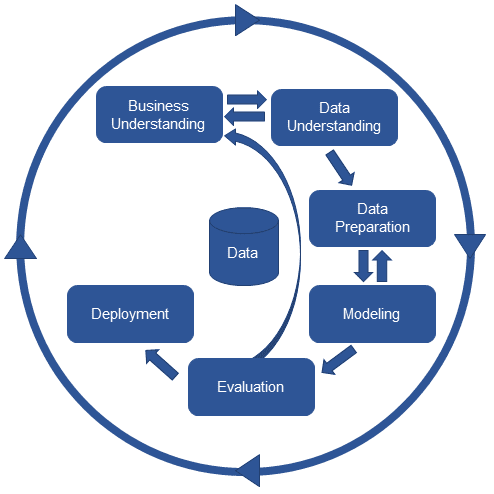![](https://www.kdnuggets.com/wp-content/uploads/crisp-dm-4-problems-fig1.png)\n    Crisp methodology is on the acceptable manners for data mining tasks. As it is belowed in the following figure, it contains three main parts should be passed to deliver a product to business\n*     Data cleaning\n        1. Understanding the business and data.\n        2. Try to comprehent the business and extract the data which is needed\n        3. Understand the dependencies between attributes. Analyzing the target variables. Handling missing values. Transforming data formats to standard data format.\n*     Data Modeling\n        1. Understanding the business and data.\n        2. Selecting more accurate classfier or regression engine based on the charactristic any of them have.\n        3. Train a model \n*     Evaluation and Deployment.\n        1. Evalute created model using evaluation methods (test-data, cross-validation, etc)\n        2. Catrefully Evaluate model with real data (i.e AB testing) (As it is shown in crisp diagram, there is a link between business undestanding and evaluation part). \n        3. Migrate to new model and replace the old one with new version.\n"},{"metadata":{"_uuid":"679d84d693888c93c63762754e36a58749be5b4d"},"cell_type":"markdown","source":"<a id=\"1\"></a> <br>\n#  2-DATA ANALYSIS\n\n\n<a id=\"3\"></a> <br>\n* **A. IMPORTS**\n\nImporting packages and libraries."},{"metadata":{"trusted":true,"_uuid":"a6430eaf18e19cc83ff3bd1a322668fde9f43f2a"},"cell_type":"code","source":"import os\nimport pandas as pd\nimport numpy as np\nimport json\nimport matplotlib.pyplot as plt\nimport datetime as datetime\nfrom datetime import timedelta, date\nimport seaborn as sns\nimport matplotlib.cm as CM\nimport lightgbm as lgb\nfrom sklearn import preprocessing\nfrom sklearn.metrics import mean_squared_error\nfrom sklearn.model_selection import GridSearchCV, train_test_split\n%matplotlib inline","execution_count":null,"outputs":[]},{"metadata":{"trusted":true,"_uuid":"86ef2c2d21767682cf351db547c3119a2339bd5e"},"cell_type":"markdown","source":"<a id=\"4\"></a> <br>\n* **B. READING DATA**\n\nReading data and caughting a glimpse of what data it is."},{"metadata":{"_cell_guid":"79c7e3d0-c299-4dcb-8224-4455121ee9b0","_uuid":"d629ff2d2480ee46fbb7e2d37f6b5fab8052498a","trusted":true},"cell_type":"code","source":"train_data = pd.read_csv(\"../input/train_v2.csv\",nrows=700000)\ntrain_data.head()","execution_count":null,"outputs":[]},{"metadata":{"trusted":true,"_uuid":"7d6396d4c5365e58dc6a10ec748cd70fce4c7c2c"},"cell_type":"code","source":"train_data.describe()","execution_count":null,"outputs":[]},{"metadata":{"trusted":true,"_uuid":"15bd454caf0148863c83b5762658f4ee2c6e7220"},"cell_type":"code","source":"list(train_data.columns.values)","execution_count":null,"outputs":[]},{"metadata":{"trusted":true,"_uuid":"2e880ed5017f078fda5067e0b17c53c980d4fea1"},"cell_type":"markdown","source":"<a id=\"5\"></a> <br>\n* **C. FEATURES DESCRIPTION**\n\nReturning back to Data description for understanding features.\n\n*     channelGrouping - The channel via which the user came to the Store.\n*     date - The date on which the user visited the Store.\n*     device - The specifications for the device used to access the Store.\n*     fullVisitorId- A unique identifier for each user of the Google Merchandise Store.\n*     geoNetwork - This section contains information about the geography of the user.\n*     sessionId - A unique identifier for this visit to the store.\n*     socialEngagementType - Engagement type, either \"Socially Engaged\" or \"Not Socially Engaged\".\n*     totals - This section contains aggregate values across the session.\n*     trafficSource - This section contains information about the Traffic Source from which the session originated.\n*     visitId - An identifier for this session. This is part of the value usually stored as the _utmb cookie. This is only unique to the user. For a completely unique ID, you should use a combination of fullVisitorId and visitId.\n*     visitNumber - The session number for this user. If this is the first session, then this is set to 1.\n*     visitStartTime - The timestamp (expressed as POSIX time).\n"},{"metadata":{"trusted":true,"_uuid":"dcb51011a920d5741ce007c15fe6f9cc122ab234"},"cell_type":"markdown","source":"<a id=\"6\"></a> <br>\n* **D. CHANNEL_GROUPING**"},{"metadata":{"trusted":true,"_uuid":"24d6d732b0e816e2a890c817dd5543ab3e5e561c"},"cell_type":"code","source":"train_data.channelGrouping.value_counts().plot(kind=\"bar\",title=\"channelGrouping distro\",figsize=(8,8),rot=25,colormap='Paired')","execution_count":null,"outputs":[]},{"metadata":{"_uuid":"98d005134d4677798e3c1431a6d95e8ac55ebe3a"},"cell_type":"markdown","source":"<a id=\"7\"></a> <br>\n* **E. DATE&VISIT_START_TIME**\n\nThere are two varialbe related to time and can be used in time dependent analyzes specially TimeSeries."},{"metadata":{"trusted":true,"_uuid":"4a21ac9e2c038995911eb25f643e157878ae9c12"},"cell_type":"code","source":"\"date :{}, visitStartTime:{}\".format(train_data.head(1).date[0],train_data.head(1).visitStartTime[0])","execution_count":null,"outputs":[]},{"metadata":{"trusted":true,"_uuid":"9426c06830d5872f44195d2f1c4acbafea4f6649"},"cell_type":"markdown","source":"date is stored in String and should be converted to pandas datetime format.\nvisitStartTime is stored in epoch unix format and should be converted to pandas datetime format.\ndoing the correspondence transforms and storing on the same attribute."},{"metadata":{"trusted":true,"_uuid":"3488ada0cedb4a6df1b205ecbc0ebe38ee2e3d40"},"cell_type":"code","source":"train_data[\"date\"] = pd.to_datetime(train_data[\"date\"],format=\"%Y%m%d\")\ntrain_data[\"visitStartTime\"] = pd.to_datetime(train_data[\"visitStartTime\"],unit='s')","execution_count":null,"outputs":[]},{"metadata":{"_uuid":"02792ece205e46a3e291572c72635b6d65c75136"},"cell_type":"markdown","source":"Checking the transformed features."},{"metadata":{"trusted":true,"_uuid":"fa57bd9f58d7b27873d7bee7913cc18ebc0e94d3"},"cell_type":"code","source":"train_data.head(1)[[\"date\",\"visitStartTime\"]]","execution_count":null,"outputs":[]},{"metadata":{"_uuid":"d2f7bc22259657a159827c45ca65972c27c55ca2"},"cell_type":"markdown","source":"<a id=\"8\"></a> <br>\n* **F. DEVICE**\n\ndevice is stored in json format. There is a need to extract its fields and analyze them. Using json library to deserializing json values."},{"metadata":{"trusted":true,"_uuid":"f0b75ca11dca15238bc3e6e6ec36e79d3d8ae90a"},"cell_type":"code","source":"list_of_devices = train_data.device.apply(json.loads).tolist()\nkeys = []\nfor devices_iter in list_of_devices:\n    for list_element in list(devices_iter.keys()):\n        if list_element not in keys:\n            keys.append(list_element)","execution_count":null,"outputs":[]},{"metadata":{"_uuid":"39d240415ddc55a1ba7744fb48662f1411828c46"},"cell_type":"markdown","source":"keys existed in device attribute are listed below.\nNow we should ignore the features which are not usefull in rest of the process. If feature is misrelated, or it contains lot of \"NaN\" values it should be discarded.\nWe select the [\"browser\",\"operatingSystem\",\"deviceCategory\",\"isMobile\"] for doing the analyzing. The rest of the device features are ignored and will be removed."},{"metadata":{"trusted":true,"_uuid":"5cd55978b512a3e1bc986a998d80a3b033c315ed"},"cell_type":"code","source":"\"keys existed in device attribute are:{}\".format(keys)","execution_count":null,"outputs":[]},{"metadata":{"trusted":true,"_uuid":"cadd6e2ecea749307f6c52056406ef9b6acbc1e2"},"cell_type":"code","source":"tmp_device_df = pd.DataFrame(train_data.device.apply(json.loads).tolist())[[\"browser\",\"operatingSystem\",\"deviceCategory\",\"isMobile\"]]","execution_count":null,"outputs":[]},{"metadata":{"trusted":true,"_uuid":"499f0847262e10fc07829916236b456364c1c472"},"cell_type":"code","source":"tmp_device_df.head()","execution_count":null,"outputs":[]},{"metadata":{"trusted":true,"_uuid":"b12bb719c32f9a7e23ab0440514149832a33a805"},"cell_type":"code","source":"tmp_device_df.describe()","execution_count":null,"outputs":[]},{"metadata":{"trusted":true,"_uuid":"1a9f91b20b7d28fd8f7efbdd0ea3ae3e2d29aea7"},"cell_type":"code","source":"fig, axes = plt.subplots(2,2,figsize=(15,15))\ntmp_device_df[\"isMobile\"].value_counts().plot(kind=\"bar\",ax=axes[0][0],rot=25,legend=\"isMobile\",color='tan')\ntmp_device_df[\"browser\"].value_counts().head(10).plot(kind=\"bar\",ax=axes[0][1],rot=40,legend=\"browser\",color='teal')\ntmp_device_df[\"deviceCategory\"].value_counts().head(10).plot(kind=\"bar\",ax=axes[1][0],rot=25,legend=\"deviceCategory\",color='lime')\ntmp_device_df[\"operatingSystem\"].value_counts().head(10).plot(kind=\"bar\",ax=axes[1][1],rot=80,legend=\"operatingSystem\",color='c')","execution_count":null,"outputs":[]},{"metadata":{"_uuid":"8fcdcdddde4e9b6c4818ea9cb46331a8f1890a70"},"cell_type":"markdown","source":"<a id=\"9\"></a> <br>\n* **G. GEO_NETWORK**\n\nIt is json and the similar manner to previous feature (device) should be done.\n"},{"metadata":{"trusted":true,"_uuid":"9d2c8de2826719ba58ca3785471aab39af56b371"},"cell_type":"code","source":"tmp_geo_df = pd.DataFrame(train_data.geoNetwork.apply(json.loads).tolist())[[\"continent\",\"subContinent\",\"country\",\"city\"]]","execution_count":null,"outputs":[]},{"metadata":{"trusted":true,"_uuid":"3e3e0826f8a489bb9642968a12f0ac7875a8c7b7"},"cell_type":"code","source":"tmp_geo_df.head()","execution_count":null,"outputs":[]},{"metadata":{"trusted":true,"_uuid":"1a750933b4507d43e92a7ce5491e5216caabfe85"},"cell_type":"code","source":"tmp_geo_df.describe()","execution_count":null,"outputs":[]},{"metadata":{"_uuid":"dba43137c32caff107e861abb03427dd5417b5d3"},"cell_type":"markdown","source":"analysing the distribution of users in 5 continents."},{"metadata":{"trusted":true,"_uuid":"c8b86fc6149849a1f78b7102edfcbb9e16cb341b"},"cell_type":"code","source":"fig, axes = plt.subplots(3,2, figsize=(15,15))\ntmp_geo_df[\"continent\"].value_counts().plot(kind=\"bar\",ax=axes[0][0],title=\"Global Distributions\",rot=0,color=\"c\")\ntmp_geo_df[tmp_geo_df[\"continent\"] == \"Americas\"][\"subContinent\"].value_counts().plot(kind=\"bar\",ax=axes[1][0], title=\"America Distro\",rot=0,color=\"tan\")\ntmp_geo_df[tmp_geo_df[\"continent\"] == \"Asia\"][\"subContinent\"].value_counts().plot(kind=\"bar\",ax=axes[0][1], title=\"Asia Distro\",rot=0,color=\"r\")\ntmp_geo_df[tmp_geo_df[\"continent\"] == \"Europe\"][\"subContinent\"].value_counts().plot(kind=\"bar\",ax=axes[1][1],  title=\"Europe Distro\",rot=0,color=\"lime\")\ntmp_geo_df[tmp_geo_df[\"continent\"] == \"Oceania\"][\"subContinent\"].value_counts().plot(kind=\"bar\",ax = axes[2][0], title=\"Oceania Distro\",rot=0,color=\"teal\")\ntmp_geo_df[tmp_geo_df[\"continent\"] == \"Africa\"][\"subContinent\"].value_counts().plot(kind=\"bar\" , ax=axes[2][1], title=\"Africa Distro\",rot=0,color=\"silver\")","execution_count":null,"outputs":[]},{"metadata":{"_uuid":"337926fa6261abcbd7fa6fd0804f300c81316a46"},"cell_type":"markdown","source":"<a id=\"10\"></a> <br>\n* **H.SOCIAL_ENGANEMENT_TYPE **\n\nDescribing this feature confirms its uniqueness. It should be dropped. Because its entropy is 0. "},{"metadata":{"trusted":true,"_uuid":"7b3911b4fee714c5f1d2c5dc2b033f7c7c7d1e01"},"cell_type":"code","source":"train_data[\"socialEngagementType\"].describe()","execution_count":null,"outputs":[]},{"metadata":{"_uuid":"24c3161564ec95f36881869b0e2f4fbf6d834b86"},"cell_type":"markdown","source":"<a id=\"11\"></a> <br>\n* **I. TOTALS**\n"},{"metadata":{"trusted":true,"_uuid":"ed05f7a083c3863e88b9d820bc10940765de245d"},"cell_type":"code","source":"train_data.head()\ntrain_data[\"revenue\"] = pd.DataFrame(train_data.totals.apply(json.loads).tolist())[[\"transactionRevenue\"]]\n","execution_count":null,"outputs":[]},{"metadata":{"_uuid":"0d6a1b3a04a6af113c0bd6ae5f75ed8ce0f6b0b3"},"cell_type":"markdown","source":"Extracting all the revenues can bring us an overview about the total revenue."},{"metadata":{"trusted":true,"_uuid":"11f9072ff0e17577979bbfee4dea7a6139bef5c8"},"cell_type":"code","source":"revenue_datetime_df = train_data[[\"revenue\" , \"date\"]].dropna()\nrevenue_datetime_df[\"revenue\"] = revenue_datetime_df.revenue.astype(np.int64)\nrevenue_datetime_df.head()","execution_count":null,"outputs":[]},{"metadata":{"_uuid":"95155bf9d934bf271a424c8a98255fc9a9194363"},"cell_type":"markdown","source":"Aggregation on days and plotting daily revenue."},{"metadata":{"trusted":true,"_uuid":"3ddbf6c05926782adbc4b6d2424e88df2c0a728a"},"cell_type":"code","source":"daily_revenue_df = revenue_datetime_df.groupby(by=[\"date\"],axis = 0 ).sum()\nimport matplotlib.pyplot as plt\nfig, axes = plt.subplots(figsize=(20,10))\naxes.set_title(\"Daily Revenue\")\naxes.set_ylabel(\"Revenue\")\naxes.set_xlabel(\"date\")\naxes.plot(daily_revenue_df[\"revenue\"])\n","execution_count":null,"outputs":[]},{"metadata":{"trusted":true,"_uuid":"a8e89d239eb5b6d510ecc8e9f17215c5bc527b16"},"cell_type":"code","source":"fig, axes = plt.subplots(nrows=1, ncols=1, figsize=(9, 9))\naxes.set_title(\"Daily revenue Violin\")\naxes.set_ylabel(\"revenue\")\naxes.violinplot(list(daily_revenue_df[\"revenue\"].values),showmeans=False,showmedians=True)","execution_count":null,"outputs":[]},{"metadata":{"_uuid":"7a1a7ed010b0ae312a18612e20fc3a4a0e78f3a8"},"cell_type":"markdown","source":"<a id=\"12\"></a> <br>\n* **J. VISIT_NUMBER**\n\nNumber of visits have profound potential to be an important factor in regression progress. "},{"metadata":{"trusted":true,"_uuid":"280d50807c7221484f954f4baef407d583d55795"},"cell_type":"code","source":"visit_datetime_df = train_data[[\"date\",\"visitNumber\"]]\nvisit_datetime_df[\"visitNumber\"] = visit_datetime_df.visitNumber.astype(np.int64)","execution_count":null,"outputs":[]},{"metadata":{"trusted":true,"_uuid":"94394db7363f82dc3e8d4b63ce04b451cfd858fa"},"cell_type":"code","source":"daily_visit_df = visit_datetime_df.groupby(by=[\"date\"], axis = 0).sum()\n\nfig, axes = plt.subplots(1,1,figsize=(20,10))\naxes.set_ylabel(\"# of visits\")\naxes.set_xlabel(\"date\")\naxes.set_title(\"Daily Visits\")\naxes.plot(daily_visit_df[\"visitNumber\"])","execution_count":null,"outputs":[]},{"metadata":{"trusted":true,"_uuid":"a19b0c54518e1b4cf2a9d40d721567c1764c6f90"},"cell_type":"code","source":"fig, axes = plt.subplots(nrows=1, ncols=1, figsize=(9, 9))\naxes.set_title(\"Daily visits Violin\")\naxes.set_ylabel(\"# of visitors\")\naxes.violinplot(list(daily_visit_df[\"visitNumber\"].values),showmeans=False,showmedians=True)","execution_count":null,"outputs":[]},{"metadata":{"_uuid":"bb23c63389e45b1a1aaba846ee8b892425d37db7"},"cell_type":"markdown","source":"Now, lets check another side of 'visitNumber' feature. As it is mentioned in data description, visitNumber is the number of sessions for each user. It can also be the factor of users interest. lets 'describe' and  'visualize' them.\nusing 'collections' package, we can count repetition of each element."},{"metadata":{"trusted":true,"_uuid":"0181ed5f1fee9854dee68331646ac2d159bfb9f4"},"cell_type":"code","source":"train_data.visitNumber.describe()","execution_count":null,"outputs":[]},{"metadata":{"_uuid":"789a4341cacf0338f8d68d9b847e94d7a8c8887b"},"cell_type":"markdown","source":"The 75% of sessions have visitNumber lower than one time. You can get more information about percentiles by calling np.percentile method."},{"metadata":{"trusted":true,"_uuid":"88e2b52a6055587655b99a59f97b24897015f59c"},"cell_type":"code","source":"\"90 percent of sessions have visitNumber lower than {} times.\".format(np.percentile(list(train_data.visitNumber),90))","execution_count":null,"outputs":[]},{"metadata":{"_uuid":"2aba10a10c0670314a0c4d5286f66b3afdc6a08d"},"cell_type":"markdown","source":"Lets find most_common and least_common visitNumbers for being familiar with collections module and its powrefull tools ;-) "},{"metadata":{"trusted":true,"_uuid":"53cbb935fed4dd082b7de40d0a6b93029dd82dc3"},"cell_type":"code","source":"import collections\n\ntmp_least_10_visitNumbers_list = collections.Counter(list(train_data.visitNumber)).most_common()[:-10-1:-1]\ntmp_most_10_visitNumbers_list = collections.Counter(list(train_data.visitNumber)).most_common(10)\nleast_visitNumbers = []\nmost_visitNumbers = []\nfor i in tmp_least_10_visitNumbers_list:\n    least_visitNumbers.append(i[0])\nfor i in tmp_most_10_visitNumbers_list:\n    most_visitNumbers.append(i[0])\n\"10 most_common visitNumbers are {} times and 10 least_common visitNumbers are {} times\".format(most_visitNumbers,least_visitNumbers)","execution_count":null,"outputs":[]},{"metadata":{"_uuid":"a69c4b314f21f0913fdf9640704802652a6f59e9"},"cell_type":"markdown","source":" It is clear that the dispersion of the 'visitNumber' per session is huge. for this sort of features, we can use Log and map the feature space to\nnew lower space. As a result of this mapping, visualization the data will be easier."},{"metadata":{"trusted":true,"_uuid":"9ff582a30ec1ec665fde671aed193095b6daf8e3"},"cell_type":"code","source":"fig,ax = plt.subplots(1,1,figsize=(9,5))\nax.set_title(\"Histogram of log(visitNumbers) \\n don't forget it is per session\")\nax.set_ylabel(\"Repetition\")\nax.set_xlabel(\"Log(visitNumber)\")\nax.grid(color='b', linestyle='-', linewidth=0.1)\nax.hist(np.log(train_data.visitNumber))","execution_count":null,"outputs":[]},{"metadata":{"_uuid":"a7aa14f5d0c7bcf8c602144bbe29821a228e6268"},"cell_type":"markdown","source":"<a id=\"13\"></a> <br>\n* **K. TRAFFIC_SOURCE**\n\nWhat is the most conventional manner for visitor who visit to the website and do their shopping ? trafficSource attribute can resolve this qurestion.\nLike a previous Json elements existed in the dataset, this attribute is also Json file. so, we use the similar way to deserialize it. We have select keyword, source and the medium as a features which can bring more useful infromation.\n"},{"metadata":{"trusted":true,"_uuid":"027a738e3c4f5a3d4066762bc66d287302470039"},"cell_type":"code","source":"traffic_source_df = pd.DataFrame(train_data.trafficSource.apply(json.loads).tolist())[[\"keyword\",\"medium\" , \"source\"]]","execution_count":null,"outputs":[]},{"metadata":{"trusted":true,"_uuid":"48e7f72f09c8ae71c3682fd8e7b47e53d3775b7a"},"cell_type":"code","source":"fig,axes = plt.subplots(1,2,figsize=(15,10))\ntraffic_source_df[\"medium\"].value_counts().plot(kind=\"bar\",ax = axes[0],title=\"Medium\",rot=0,color=\"tan\")\ntraffic_source_df[\"source\"].value_counts().head(10).plot(kind=\"bar\",ax=axes[1],title=\"source\",rot=75,color=\"teal\")","execution_count":null,"outputs":[]},{"metadata":{"trusted":true,"_uuid":"df8a4d663158bcc3a00568a41c4ec3fc5fefb7c7"},"cell_type":"markdown","source":"As it is completely obvious in source diagram, google is the most repetitive source. It would be interesting if we replace all google subdomains with exact 'google' and do the same analyze again. let's do it."},{"metadata":{"trusted":true,"_uuid":"c1e14eb231912f233cadb2bb0ba48e0ce64b4366"},"cell_type":"code","source":"traffic_source_df.loc[traffic_source_df[\"source\"].str.contains(\"google\") ,\"source\"] = \"google\"\nfig,axes = plt.subplots(1,1,figsize=(8,8))\ntraffic_source_df[\"source\"].value_counts().head(15).plot(kind=\"bar\",ax=axes,title=\"source\",rot=75,color=\"teal\")","execution_count":null,"outputs":[]},{"metadata":{"trusted":true,"_uuid":"32f46b9faea7670aafecf55b922bb2df0ef8d0c0"},"cell_type":"markdown","source":"Google dependent redirects are more than twice the youtube sources. Combination of this feature with revenue and visits may have important result. We will do it in next step (when we are analyzing feature correlations).\nNow let's move on keywords feature.\nA glance to keyword featre represnets lot of missing values '(not provided)'. Drawing a bar chart for both of them...\n"},{"metadata":{"trusted":true,"_uuid":"4f0703fa5288ee3e0570f30aefb2739761ce66bd"},"cell_type":"code","source":"fig,axes = plt.subplots(1,2,figsize=(15,10))\ntraffic_source_df[\"keyword\"].value_counts().head(10).plot(kind=\"bar\",ax=axes[0], title=\"keywords (total)\",color=\"orange\")\ntraffic_source_df[traffic_source_df[\"keyword\"] != \"(not provided)\"][\"keyword\"].value_counts().head(15).plot(kind=\"bar\",ax=axes[1],title=\"keywords (dropping NA)\",color=\"c\")","execution_count":null,"outputs":[]},{"metadata":{"_uuid":"d47e98109052c593a71437ab8c28d4cfcd674569"},"cell_type":"markdown","source":"<a id=\"14\"></a> <br>\n* **L. FULL_VISITOR_ID**\n\nNow, lets see how many of users are repetitive ?! This feature can represent important information answering this question ? (Is more repeation proportional to more buy ?! ) \nThe response will be discussed in next section (Where we are analyzing compound features) but now, lets move on calculation of repetitive visits percentiles."},{"metadata":{"trusted":true,"_uuid":"25a3dc6ee29147c2af2037e3b167f84bcf724183"},"cell_type":"code","source":"repetitive_users = list(np.sort(list(collections.Counter(list(train_data[\"fullVisitorId\"])).values())))\n\"25% percentile: {}, 50% percentile: {}, 75% percentile: {}, 88% percentile: {}, 88% percentile: {}\".format(\nnp.percentile(repetitive_users,q=25),np.percentile(repetitive_users,q=50),\nnp.percentile(repetitive_users,q=75),np.percentile(repetitive_users,q=88), np.percentile(repetitive_users,q=89))","execution_count":null,"outputs":[]},{"metadata":{"_uuid":"338ab31e3cc9cf9301225f999020888394025edb"},"cell_type":"markdown","source":"As it is shown, only 12 percent of users are repetitive and visited the website more than once. \n(Search about churn rate and conversion rate if you want to know why we have analyzed this feature ;-) )\n"},{"metadata":{"trusted":true,"_uuid":"89a7f318e36ea214cb77777bb09e3ceaf3d6a591"},"cell_type":"markdown","source":"#  3-COMPOUND FEATURES\n\n<a id=\"16\"></a> <br>\n* **A. CHURN&CONVERSION_VISUALIZATION**\n\nThe main definition of ChurnRate is The percentage rate at which customers stop subscribing to a service or employees leave a job. Churn rate period can be various from day to a year correspoding to business type. In this section, we will compute and visualize the monthly churn rate. \nLets do more investigation on features date and fullVisitorId for more detail mining.\n"},{"metadata":{"trusted":true,"_uuid":"3aecd41e62d35ee288e6f8194b8a15b4fee7e145"},"cell_type":"code","source":"date_list = np.sort(list(set(list(train_data[\"date\"]))))\n\"first_day:'{}' and last_day:'{}' and toal number of data we have is: '{}' days.\".format(date_list[0], date_list[-1],len(set(list(train_data[\"date\"]))))","execution_count":null,"outputs":[]},{"metadata":{"_uuid":"504213d4e82a108eafe96340236c61929e27836d"},"cell_type":"markdown","source":"So, we have 366 days (12 month = 1 year) from August 2016  to August 2017  data for churn rate calculations. The bes period for churn maybe is the monthly churn rate.\nNow, lets list all the months existed in library for checking having no missing months."},{"metadata":{"trusted":true,"_uuid":"d0b87c3fb522149f972888671047b1d9608d033e"},"cell_type":"code","source":"month = 8\nstart_date = datetime.date(2016, month, 1)\nend_date = datetime.date(2017, month, 1)\ndef daterange(start_date, end_date):\n    for n in range(int((end_date - start_date).days)):\n        yield start_date + timedelta(n)\ndates_month = []\nfor single_date in daterange(start_date, end_date):\n    dates_month.append(single_date.strftime(\"%Y-%m\"))\ndates_month = list(set(dates_month))\ndates_month","execution_count":null,"outputs":[]},{"metadata":{"_uuid":"cddac95d8be2bd4a1eb951a260f4aefa4a32896a"},"cell_type":"markdown","source":"Whole the period exist in data. So, Lets define new empty dataframe and do this calculations on it and copy the our requirements ot it.\nfor churn rate calculations, we need to check which users visited have visited the website monthly. this information is located in fullVisitorId. we will copy it to new df."},{"metadata":{"trusted":true,"_uuid":"dc25de8cdbf95d0d7e6bf3d5f7f212035b9b6ee4"},"cell_type":"code","source":"tmp_churn_df = pd.DataFrame()\ntmp_churn_df[\"date\"] = train_data[\"date\"]\ntmp_churn_df[\"yaer\"] = pd.DatetimeIndex(tmp_churn_df[\"date\"]).year\ntmp_churn_df[\"month\"] =pd.DatetimeIndex(tmp_churn_df[\"date\"]).month\ntmp_churn_df[\"fullVisitoId\"] = train_data[\"fullVisitorId\"]\ntmp_churn_df.head()","execution_count":null,"outputs":[]},{"metadata":{"_uuid":"6510f3a5700041d334b60731565e2757e03a52d0"},"cell_type":"markdown","source":"For calculation of churn rate we need to count the users appeared in two, three, four, etc. continus months. \nWe will using the following format for collocation of users. \nFor example assume we want to extract the number of distinct users who visited the website on 2016-08."},{"metadata":{"trusted":true,"_uuid":"b265e974d9adef4f2eba1e829a345e76c66aef0b"},"cell_type":"code","source":"\"distinct users who visited the website on 2016-08 are:'{}'persons\".format(len(set(tmp_churn_df[(tmp_churn_df.yaer == 2016) & (tmp_churn_df.month == 8) ][\"fullVisitoId\"])))","execution_count":null,"outputs":[]},{"metadata":{"_uuid":"d5e0e7dac39dd4b15b1c84c6461a129976ee90ed"},"cell_type":"markdown","source":"By generalizing the above solution we have:"},{"metadata":{"trusted":true,"_uuid":"1eb62cdcfbe01828f8ee4b9e8c1e34c3b1ba73a5"},"cell_type":"code","source":"target_intervals_list = [(2016,8),(2016,9),(2016,10),(2016,11),(2016,12),(2017,1),(2017,2),(2017,3),(2017,4),(2017,5),(2017,6),(2017,7)]\nintervals_visitors = []\nfor tmp_tuple in target_intervals_list:\n    intervals_visitors.append(tmp_churn_df[(tmp_churn_df.yaer == tmp_tuple[0]) & (tmp_churn_df.month == tmp_tuple[1]) ][\"fullVisitoId\"])\n\"Size of intervals_visitors:{} \".format(len(intervals_visitors))","execution_count":null,"outputs":[]},{"metadata":{"_uuid":"aeecd93d97a70f54885e4841c1d8866ad065b520"},"cell_type":"markdown","source":"So, we have 12 list and each elemets contains the users who visited the website on the correspondence period.\nNow its time to do some matrix calculation for filling the churn-rate matrix.\nIt is very probable that you calculate the matrix with more efficient ways. I used this manner for more simplicity."},{"metadata":{"trusted":true,"_uuid":"b844e618c9beb2bf76be68ac13c6c7fb20b6263e"},"cell_type":"code","source":"tmp_matrix = np.zeros((11,11))\n\nfor i in range(0,11):\n    k = False\n    tmp_set = []\n    for j in range(i,11): \n        if k:\n            tmp_set = tmp_set & set(intervals_visitors[j])\n        else:\n            tmp_set = set(intervals_visitors[i]) & set(intervals_visitors[j])\n        tmp_matrix[i][j] = len(list(tmp_set))\n        k = True","execution_count":null,"outputs":[]},{"metadata":{"_uuid":"64f1ae0db9049c9cda12afb17386eb9e380ecf6c"},"cell_type":"markdown","source":"Now we have 2D matrix containig the continus visited users."},{"metadata":{"trusted":true,"_uuid":"bb0ec2429438226f82b5bd7dd08e0e610c00f6fb"},"cell_type":"code","source":"xticklabels = [\"interval 1\",\"interval 2\",\"interval 3\",\"interval 4\",\"interval 5\",\"interval 6\",\"interval 7\",\"interval 8\",\n              \"interval 9\",\"interval 10\",\"interval 11\"]\nyticklabels = [(2016,8),(2016,9),(2016,10),(2016,11),(2016,12),(2017,1),(2017,2),(2017,3),(2017,4),(2017,5),(2017,6),(2017,7)]\nfig, ax = plt.subplots(figsize=(11,11))\nax = sns.heatmap(np.array(tmp_matrix,dtype=int), annot=True, cmap=\"RdBu_r\",xticklabels=xticklabels,fmt=\"d\",yticklabels=yticklabels)\nax.set_title(\"Churn-rate heatmap\")\nax.set_xlabel(\"intervals\")\nax.set_ylabel(\"months\")\n","execution_count":null,"outputs":[]},{"metadata":{"_uuid":"5acd00596bd46ac286484a1bac0c9a3b3c9de9b1"},"cell_type":"markdown","source":"A churn-rate heat map is the one the important keys of business. The more repetitive users in continues time periods, the more success in user loyalty.\n\nGeneraly it is better to drop the zeors below the main diagonal for better visualization and more clearer representaion. \n(I couldn't find the sns pleasant visualization for half churn rate matrix. If you find it, it will be appreciated to ping me. Ill replace the below diagram with your recommendation as soon as possible)."},{"metadata":{"trusted":true,"_uuid":"7786164b7ad678c1bb7de2e699ade662d6920763"},"cell_type":"code","source":"A = tmp_matrix\nmask =  np.tri(A.shape[0], k=-1)\nA = np.ma.array(A, mask=mask) # mask out the lower triangle\nfig = plt.figure(figsize=(9,9))\nax = fig.add_subplot(111)\nax.set_xlabel(\"interval\")\nax.set_ylabel(\"period\")\ncmap = CM.get_cmap('RdBu_r', 50000) \ncmap.set_bad('w') # default value is 'k'\nax.imshow(A, interpolation=\"nearest\", cmap=cmap)","execution_count":null,"outputs":[]},{"metadata":{"_uuid":"ba8655158e0f81976b6691dbe3377602c07e4c0a"},"cell_type":"markdown","source":"\n<a id=\"17\"></a> <br>\n* **B. REVENUE&DATETIME**\n\n\nNow, it is time to move on to analysing compound features. The main target of this section is undestanding the features correlation. \nAt the first point, lets analyze this probable assumption :\n\n\"Is more visitNumber proportional to more Revenue ?!\"\n"},{"metadata":{"trusted":true,"_uuid":"d5c53baecad877d02711d142b8803a9eb1348332"},"cell_type":"code","source":"revenue_datetime_df = train_data[[\"revenue\" , \"date\"]].dropna()\nrevenue_datetime_df[\"revenue\"] = revenue_datetime_df.revenue.astype(np.int64)\nrevenue_datetime_df.head()","execution_count":null,"outputs":[]},{"metadata":{"_kg_hide-input":true,"_uuid":"1a048dc239959ec71029c2d1ecd4e9b97d05d293"},"cell_type":"markdown","source":"Doing groupby on date and getting the total revenue per day:"},{"metadata":{"trusted":true,"_uuid":"5fe90fc6b104f1b0586cd196ee3bbe43febc6931"},"cell_type":"code","source":"total_revenue_daily_df = revenue_datetime_df.groupby(by=[\"date\"],axis=0).sum()\ntotal_revenue_daily_df.head()","execution_count":null,"outputs":[]},{"metadata":{"_uuid":"ca1d6f05bf4befad1e755950c89b7c2b21540926"},"cell_type":"markdown","source":"Doing similar process on visitNumber and getting total visitNumber per day."},{"metadata":{"trusted":true,"_uuid":"2c37cd5e4b5feb8bc3b99865c1e1a78c309ab0d9"},"cell_type":"code","source":"total_visitNumber_daily_df = train_data[[\"date\",\"visitNumber\"]].groupby(by=[\"date\"],axis=0).sum()\ntotal_visitNumber_daily_df.head()","execution_count":null,"outputs":[]},{"metadata":{"_uuid":"44698a25f7eebdeb67da3ca2c1ba2ddded9c06c3"},"cell_type":"markdown","source":"Concatenate these two dataframe and compound visualization."},{"metadata":{"trusted":true,"_uuid":"e1eddb7ab69446da5566340ecd4a319cbffbc55e"},"cell_type":"code","source":"datetime_revenue_visits_df = pd.concat([total_revenue_daily_df,total_visitNumber_daily_df],axis=1)\n\nfig, ax1 = plt.subplots(figsize=(20,10))\nt = datetime_revenue_visits_df.index\ns1 = datetime_revenue_visits_df[\"visitNumber\"]\nax1.plot(t, s1, 'b-')\nax1.set_xlabel('day')\n# Make the y-axis label, ticks and tick labels match the line color.\nax1.set_ylabel('visitNumber', color='b')\nax1.tick_params('y', colors='b')\n\nax2 = ax1.twinx()\ns2 = datetime_revenue_visits_df[\"revenue\"]\nax2.plot(t, s2, 'r--')\nax2.set_ylabel('revenue', color='r')\nax2.tick_params('y', colors='r')\nfig.tight_layout()","execution_count":null,"outputs":[]},{"metadata":{"_uuid":"df6a04b932bd865c1eec26b0b7edf621fbca6652"},"cell_type":"markdown","source":"By comparing the revenue and visitNumbers we can confirm our consumption. Where there is more visit the revenue is also more than neighbour days.\nThe behaviour of line charts is completely similar.\n\nAnother point to touch on is the rate of visitNumber and revenue  which have a peak on December. Before christmas people visit and buy more than other days. The same behaviour is represented in the days after christmas where people have bought their requirements and the level of visit and buy goes down (They are in vacation and have less time to check the website ;-) )\n\nThe above diagram can be represent more detail if you visualize period of it. Do it yourself with by quering on daterange and check our confirmed assumtion :-D."},{"metadata":{"_uuid":"792e4f71aad4e7f5d86457cf62364c4dd29653d2"},"cell_type":"markdown","source":"Lets focus on user who have addressed our challenge (users who have revenue) and checking some assumptions"},{"metadata":{"trusted":true,"_uuid":"f09aa84f3fcbc907ed13145ac232449808a5088f"},"cell_type":"code","source":"revenue_df = train_data.dropna(subset=[\"revenue\"])\nrevenue_os_df = pd.DataFrame(revenue_df.device.apply(json.loads).tolist())[[\"browser\",\"operatingSystem\",\"deviceCategory\",\"isMobile\"]]\n\nbuys_is_mobile_dict = dict(collections.Counter(list(revenue_os_df.isMobile)))\npercent_buys_is_mobile_dict = {k: v / total for total in (sum(buys_is_mobile_dict.values()),) for k, v in buys_is_mobile_dict.items()}\nsizes = list(percent_buys_is_mobile_dict.values())\nexplode=(0,0.1)\nlabels = 'isNotMobile', 'isMobile'\nfig, ax = plt.subplots(1,1, figsize=(8,8))\nax.set_title(\"buys mobile distro\")\nax.pie(sizes, explode=explode, labels=labels, autopct='%1.1f%%',shadow=True, startangle=90)","execution_count":null,"outputs":[]},{"metadata":{"_uuid":"d87db6c6826d5070c13dfec70744c65c17480c2b"},"cell_type":"markdown","source":"Going deeper to subclasses ..."},{"metadata":{"trusted":true,"_uuid":"94d501a18ab2cba0b084054563891ea10ce496c1","scrolled":true},"cell_type":"code","source":"mobiles_browsers = dict(collections.Counter(revenue_os_df[revenue_os_df[\"isMobile\"] == True][\"browser\"]))\nnot_mobiles_browsers = dict(collections.Counter(revenue_os_df[revenue_os_df[\"isMobile\"] == False][\"browser\"]))\nprint(\"for mobile users:\")\nfor i,v in mobiles_browsers.items():\n    print(\"{}:{}\".format(i,v))\nprint(\"\\nfor not mobile users:\")\nfor i,v in not_mobiles_browsers.items():\n    print(\"{}:{}\".format(i,v))\nvals = np.array([[552.,6.,2.,12.,16.,431.], [9801.,189.,58.,93.,5.,349.]])\n\nfig, ax = plt.subplots(subplot_kw=dict(polar=True),figsize=(9,9))\nsize = 0.3\nvalsnorm = vals / np.sum(vals) * 2 * np.pi\n\n# obtain the ordinates of the bar edges\nvalsleft = np.cumsum(np.append(0, valsnorm.flatten()[:-1])).reshape(vals.shape)\n\ncmap = plt.get_cmap(\"tab20c\")\nouter_colors = cmap(np.arange(3) * 4)\ninner_colors = cmap(np.array([1, 2, 5, 6, 9, 10]))\n\nax.bar(x=valsleft[:, 0],\n       width=valsnorm.sum(axis=1), bottom=1 - size, height=size,\n       color=outer_colors, edgecolor='w', linewidth=1, align=\"edge\")\n\nax.bar(x=valsleft.flatten(),\n       width=valsnorm.flatten(), bottom=1 - 2 * size, height=size,\n       color=inner_colors, edgecolor='w', linewidth=1, align=\"edge\")\n# ax.set_axis_off()\n\nax.set(title=\"Nested pi-plot for buyers devices.\")","execution_count":null,"outputs":[]},{"metadata":{"_uuid":"d6c8ce4ae2af1e892a2e5a3d3be74ccba12618fb"},"cell_type":"markdown","source":"For buyers who use mobile for purchasing, Safari and chrome approximately have equal number of users. But for users who do not use mobile for purchasing, Safari have a few percent of total users. "},{"metadata":{"_uuid":"0880a45beba53b8f8d4a1af54ef6ab52ed89a548"},"cell_type":"markdown","source":"<a id=\"18\"></a> <br>\n#  4-BASIC REGRESSION\n\nNow, based on the analysis we have done, it's time to start the regression progress.\nLets do a simple regression for testing our regression method.\nCalling our main_df and dropping the features that may have not any positive effect on the regression results ( HINT: consider it is starting point. We want to learn how we can use the regression for combination of categorical features and continus features. We will change our features in next steps for getting better results).\nWe use the tricks we used during this tutorial for dealing with features."},{"metadata":{"trusted":true,"_uuid":"b3adcc9a0d69e50089384929b359f7c3ffbf3ed6"},"cell_type":"code","source":"df_train = train_data.drop([\"date\", \"socialEngagementType\", \"visitStartTime\", \"visitId\", \"fullVisitorId\" , \"revenue\",\"customDimensions\"], axis=1)\n\ndevices_df = pd.DataFrame(df_train.device.apply(json.loads).tolist())[[\"browser\", \"operatingSystem\", \"deviceCategory\", \"isMobile\"]]\ngeo_df = pd.DataFrame(df_train.geoNetwork.apply(json.loads).tolist())[[\"continent\", \"subContinent\", \"country\", \"city\"]]\ntraffic_source_df = pd.DataFrame(df_train.trafficSource.apply(json.loads).tolist())[[\"keyword\", \"medium\", \"source\"]]\ntotals_df = pd.DataFrame(df_train.totals.apply(json.loads).tolist())[[\"transactionRevenue\", \"newVisits\", \"bounces\", \"pageviews\", \"hits\"]]\n\n\ndf_train = pd.concat([df_train.drop([\"hits\"],axis=1), devices_df, geo_df, traffic_source_df, totals_df], axis=1)\ndf_train = df_train.drop([\"device\", \"geoNetwork\", \"trafficSource\", \"totals\"], axis=1)\n","execution_count":null,"outputs":[]},{"metadata":{"trusted":true,"_uuid":"4ac3da5624dc46c18fc5ae39c8365411d859cdbd"},"cell_type":"code","source":"df_train.head(1)","execution_count":null,"outputs":[]},{"metadata":{"_uuid":"c0467b40c1cca0df9cc2f58baacd4bce770efc72"},"cell_type":"markdown","source":"Replacing NaN variables with 0 (It may have positive/negative effect. We will check it later).\nAnother point we must touch on is we need to convert"},{"metadata":{"_uuid":"3f50dd46169c630328557f814c0e38476fd15a73","trusted":true},"cell_type":"code","source":"df_train[\"transactionRevenue\"] = df_train[\"transactionRevenue\"].fillna(0)\ndf_train[\"bounces\"] = df_train[\"bounces\"].fillna(0)\ndf_train[\"pageviews\"] = df_train[\"pageviews\"].fillna(0)\ndf_train[\"hits\"] = df_train[\"hits\"].fillna(0)\ndf_train[\"newVisits\"] = df_train[\"newVisits\"].fillna(0)","execution_count":null,"outputs":[]},{"metadata":{"_uuid":"09d288e14bc0e9d9d98fa31b500f050be68e2ce1"},"cell_type":"markdown","source":"Using train_test_split for splitting data to train and evaluate sets. Converting revenue (our target variable) to float for performing regression."},{"metadata":{"trusted":true,"_uuid":"ff52b66f6ba4d2874ecaf7aab14028dfbe01d9df"},"cell_type":"code","source":"df_train, df_test = train_test_split(df_train, test_size=0.2, random_state=42)\n\ndf_train[\"transactionRevenue\"] = df_train[\"transactionRevenue\"].astype(np.float)\ndf_test[\"transactionRevenue\"] = df_test[\"transactionRevenue\"].astype(np.float)\n\"Finaly, we have these columns for our regression problems: {}\".format(df_train.columns)","execution_count":null,"outputs":[]},{"metadata":{"trusted":true,"_uuid":"a7715a788b5ee41e377d82078f40b0378ee9e844"},"cell_type":"code","source":"df_train.head(1)","execution_count":null,"outputs":[]},{"metadata":{"_uuid":"29ea798cce627e29cac6a9c1d458a45a8a7ef00d"},"cell_type":"markdown","source":"Another point to touch on is we need to convert our categorical data to (int) values. As a result regression algorithm and classifiers can deal with these sort of features ( String features are not supported).\n(Search about LabelEncoder and its use case. This tool helps us to convert the categorical features to Integer ones)."},{"metadata":{"trusted":true,"_uuid":"dbd00b141e9796c80379034f41324a0ff8879b5d"},"cell_type":"code","source":"categorical_features = ['channelGrouping', 'browser', 'operatingSystem', 'deviceCategory', 'isMobile',\n                        'continent', 'subContinent', 'country', 'city', 'keyword', 'medium', 'source']\n\nnumerical_features = ['visitNumber', 'newVisits', 'bounces', 'pageviews', 'hits']\n\nfor column_iter in categorical_features:\n    lbl = preprocessing.LabelEncoder()\n    lbl.fit(list(df_train[column_iter].values.astype('str')) + list(df_test[column_iter].values.astype('str')))\n    df_train[column_iter] = lbl.transform(list(df_train[column_iter].values.astype('str')))\n    df_test[column_iter] = lbl.transform(list(df_test[column_iter].values.astype('str')))\n\nfor column_iter in numerical_features:\n    df_train[column_iter] = df_train[column_iter].astype(np.float)\n    df_test[column_iter] = df_test[column_iter].astype(np.float)","execution_count":null,"outputs":[]},{"metadata":{"_uuid":"96deaf50b6a81e0eee438146b01e44c126a5f738"},"cell_type":"markdown","source":"OK. Now we have all requirements which are needed for first regression test ;-).\n\nCheck [this link](http://github.com/Microsoft/LightGBM/tree/master/examples/python-guide) out for get more information about Regression algorithm we are using.\n\nIt is mentioned in competition description that we need to use ln(x+1) for evaluation of results. So, check [this links](https://docs.scipy.org/doc/numpy-1.15.1/reference/generated/numpy.log1p.html) and [this link](https://docs.scipy.org/doc/numpy-1.13.0/reference/generated/numpy.expm1.html) about these scipy built-in methods.\nWe can control prints with 'verbose_eval' parameter."},{"metadata":{"trusted":true,"_uuid":"a2a2fc640d4da78291252d6e079147a176506d77"},"cell_type":"code","source":"params = {\n    \"objective\": \"regression\",\n    \"metric\": \"rmse\",\n    \"num_leaves\": 30,\n    \"min_child_samples\": 100,\n    \"learning_rate\": 0.1,\n    \"bagging_fraction\": 0.7,\n    \"feature_fraction\": 0.5,\n    \"bagging_frequency\": 5,\n    \"bagging_seed\": 2018,\n    \"verbosity\": -1\n}\nlgb_train = lgb.Dataset(df_train.loc[:,df_train.columns != \"transactionRevenue\"], np.log1p(df_train.loc[:,\"transactionRevenue\"]))\nlgb_eval = lgb.Dataset(df_test.loc[:,df_test.columns != \"transactionRevenue\"], np.log1p(df_test.loc[:,\"transactionRevenue\"]), reference=lgb_train)\ngbm = lgb.train(params, lgb_train, num_boost_round=2000, valid_sets=[lgb_eval], early_stopping_rounds=100,verbose_eval=100)","execution_count":null,"outputs":[]},{"metadata":{"_uuid":"ebd4453a8261f116b641671793264ab3d6e9640b"},"cell_type":"markdown","source":"Congrate ! \nYou get reasonable rmse in first step. Now, lets predict the revenues for our evaluation dataset to be familar with transformation needed.\n\n(Point that the revenue of user cant be negative ;-) so, remove them)."},{"metadata":{"trusted":true,"_uuid":"4ae51a08b3f9dc61f18083fde4c9abd04ccac70b"},"cell_type":"code","source":"predicted_revenue = gbm.predict(df_test.loc[:,df_test.columns != \"transactionRevenue\"], num_iteration=gbm.best_iteration)\npredicted_revenue[predicted_revenue < 0] = 0 \ndf_test[\"predicted\"] = np.expm1(predicted_revenue)\ndf_test[[\"transactionRevenue\",\"predicted\"]].head(10)","execution_count":null,"outputs":[]},{"metadata":{"_uuid":"a66388ab5b448072538e4a9f3929d22b75147f15"},"cell_type":"markdown","source":"Now, you can generalize this procedure and use do your submission.\n\nWe will try to do a more supervised regression in next steps. We will utilize our preprocess facts for getting regression results with less error."},{"metadata":{"_uuid":"8f614d7c9535213661d1ec54ae35f7eb19551299"},"cell_type":"markdown","source":"<a id=\"19\"></a> <br>\n#  5-PREPARING FOR MORE EVALUATIONS AND TESTS\n\nNow, we have all requirements for doing more tests. Lets summarize all the prcess we have done earlier in one script. You can change parameters regarding your understanding about feature engineering process. If you cant understand any section of it, please read the details which are described below."},{"metadata":{"trusted":true,"_uuid":"9b20b5fbccaf2a71c72db5c11db19b1a7ccf775c"},"cell_type":"code","source":"import gc; gc.collect()\nimport time; time.sleep(5)\n\ndf_train = pd.read_csv(filepath_or_buffer=\"../input/train_v2.csv\",nrows=50000)\ndf_actual_test = pd.read_csv(filepath_or_buffer=\"../input/test_v2.csv\",nrows=25000)\n\n# drop useless features => date, fullVisitorId, sessionId, socialEngagement, visitStartTime\ndf_train = df_train.drop([\"date\", \"socialEngagementType\", \"visitStartTime\", \"visitId\", \"fullVisitorId\"], axis=1)\ndf_actual_test = df_actual_test.drop([\"date\", \"socialEngagementType\", \"visitStartTime\", \"visitId\"], axis=1)\n\n\n#preprocessing for trains\ndevices_df = pd.DataFrame(df_train.device.apply(json.loads).tolist())[[\"browser\", \"operatingSystem\", \"deviceCategory\", \"isMobile\"]]\ngeo_df = pd.DataFrame(df_train.geoNetwork.apply(json.loads).tolist())[[\"continent\", \"subContinent\", \"country\", \"city\"]]\ntraffic_source_df = pd.DataFrame(df_train.trafficSource.apply(json.loads).tolist())[[\"keyword\", \"medium\", \"source\"]]\ntotals_df = pd.DataFrame(df_train.totals.apply(json.loads).tolist())[[\"transactionRevenue\", \"newVisits\", \"bounces\", \"pageviews\", \"hits\"]]\ndf_train = pd.concat([df_train.drop([\"hits\"],axis=1), devices_df, geo_df, traffic_source_df, totals_df], axis=1)\ndf_train = df_train.drop([\"device\", \"geoNetwork\", \"trafficSource\", \"totals\"], axis=1)\ndf_train[\"transactionRevenue\"] = df_train[\"transactionRevenue\"].fillna(0)\ndf_train[\"bounces\"] = df_train[\"bounces\"].fillna(0)\ndf_train[\"pageviews\"] = df_train[\"pageviews\"].fillna(0)\ndf_train[\"hits\"] = df_train[\"hits\"].fillna(0)\ndf_train[\"newVisits\"] = df_train[\"newVisits\"].fillna(0)\n\n#preprocessing for tests\ndevices_df = pd.DataFrame(df_actual_test.device.apply(json.loads).tolist())[[\"browser\", \"operatingSystem\", \"deviceCategory\", \"isMobile\"]]\ngeo_df = pd.DataFrame(df_actual_test.geoNetwork.apply(json.loads).tolist())[[\"continent\", \"subContinent\", \"country\", \"city\"]]\ntraffic_source_df = pd.DataFrame(df_actual_test.trafficSource.apply(json.loads).tolist())[[\"keyword\", \"medium\", \"source\"]]\ntotals_df = pd.DataFrame(df_actual_test.totals.apply(json.loads).tolist())[[\"newVisits\", \"bounces\", \"pageviews\", \"hits\"]]\ndf_actual_test = pd.concat([df_actual_test.drop([\"hits\"],axis=1), devices_df, geo_df, traffic_source_df, totals_df], axis=1)\ndf_actual_test = df_actual_test.drop([\"device\", \"geoNetwork\", \"trafficSource\", \"totals\"], axis=1)\n# df_actual_test[\"transactionRevenue\"] = df_train[\"transactionRevenue\"].fillna(0)\ndf_actual_test[\"bounces\"] = df_train[\"bounces\"].fillna(0)\ndf_actual_test[\"pageviews\"] = df_train[\"pageviews\"].fillna(0)\ndf_actual_test[\"hits\"] = df_train[\"hits\"].fillna(0)\ndf_actual_test[\"newVisits\"] = df_train[\"newVisits\"].fillna(0)\n\n#garbage collector ';-)'\ndel devices_df,geo_df,traffic_source_df,totals_df\n\n\n#evaluation \ndf_train, df_eval = train_test_split(df_train, test_size=0.2, random_state=42)\n\n# lgb_train = lgb.Dataset(df_train.loc[:, df_train.columns != \"revenue\"], df_train[\"revenue\"])\n# lgb_eval = lgb.Dataset(df_test.loc[:, df_test.columns != \"revenue\"], df_test[\"revenue\"], reference=lgb_train)\n\ndf_train[\"transactionRevenue\"] = df_train[\"transactionRevenue\"].astype(np.float)\ndf_eval[\"transactionRevenue\"] = df_eval[\"transactionRevenue\"].astype(np.float)\n\nprint(df_train.columns)","execution_count":null,"outputs":[]},{"metadata":{"_uuid":"7422339fe51434aa3f9a35e866fa4f12b3a01eda","trusted":true},"cell_type":"code","source":"params = {\n    \"objective\": \"regression\",\n    \"metric\": \"rmse\",\n    \"num_leaves\": 30,\n    \"min_child_samples\": 100,\n    \"learning_rate\": 0.1,\n    \"bagging_fraction\": 0.7,\n    \"feature_fraction\": 0.5,\n    \"bagging_frequency\": 5,\n    \"bagging_seed\": 2018,\n    \"verbosity\": -1\n}\n\nprint('Start training...')","execution_count":null,"outputs":[]},{"metadata":{"trusted":true,"_uuid":"a48f07cf051a84064969a1a3cb563aec42bf6738"},"cell_type":"code","source":"df_actual_test = df_actual_test.drop([\"customDimensions\"],axis=1)\ndf_train = df_train.drop([\"customDimensions\"],axis=1)\ndf_eval = df_eval.drop([\"customDimensions\"],axis=1)","execution_count":null,"outputs":[]},{"metadata":{"trusted":true,"_uuid":"765541d7b167588704e56d13efd31d323e0c77b6"},"cell_type":"code","source":"categorical_features = ['channelGrouping', 'browser', 'operatingSystem', 'deviceCategory', 'isMobile',\n                        'continent', 'subContinent', 'country', 'city', 'keyword', 'medium', 'source']\n\nnumerical_features = ['visitNumber', 'newVisits', 'bounces', 'pageviews', 'hits']\n\nfor column_iter in categorical_features:\n    lbl = preprocessing.LabelEncoder()\n    lbl.fit(list(df_train[column_iter].values.astype('str')) + list(df_eval[column_iter].values.astype('str')) + list(df_actual_test[column_iter].values.astype('str')))\n    \n    df_train[column_iter] = lbl.transform(list(df_train[column_iter].values.astype('str')))\n    df_eval[column_iter] = lbl.transform(list(df_eval[column_iter].values.astype('str')))\n    df_actual_test[column_iter] = lbl.transform(list(df_actual_test[column_iter].values.astype('str')))\n\nfor column_iter in numerical_features:\n    df_train[column_iter] = df_train[column_iter].astype(np.float)\n    df_eval[column_iter] = df_eval[column_iter].astype(np.float)\n    df_actual_test[column_iter] = df_actual_test[column_iter].astype(np.float)","execution_count":null,"outputs":[]},{"metadata":{"trusted":true,"_uuid":"c6962025557a22ea96b7297fd7f1fe260f219192"},"cell_type":"code","source":"lgb_train = lgb.Dataset(df_train.loc[:,df_train.columns != \"transactionRevenue\"], np.log1p(df_train.loc[:,\"transactionRevenue\"]))\nlgb_eval = lgb.Dataset(df_eval.loc[:,df_eval.columns != \"transactionRevenue\"], np.log1p(df_eval.loc[:,\"transactionRevenue\"]), reference=lgb_train)","execution_count":null,"outputs":[]},{"metadata":{"trusted":true,"_uuid":"9fb8a62b7dd7d8597201ef894a56eeb60c3fcb82"},"cell_type":"code","source":"gbm = lgb.train(params, lgb_train, num_boost_round=2000, valid_sets=[lgb_eval], early_stopping_rounds=100,verbose_eval=100)","execution_count":null,"outputs":[]},{"metadata":{"trusted":true,"_uuid":"b89a7709181c01f83a91f46a50cff5578f755a47"},"cell_type":"code","source":"eval_predicted_revenue = gbm.predict(df_eval.loc[:,df_eval.columns != \"transactionRevenue\"], num_iteration=gbm.best_iteration)\neval_predicted_revenue[eval_predicted_revenue < 0] = 0 \ndf_eval[\"predicted\"] = np.expm1(eval_predicted_revenue)\ndf_eval[[\"transactionRevenue\",\"predicted\"]].head()","execution_count":null,"outputs":[]},{"metadata":{"trusted":true,"_uuid":"aae37660a0f72dc4647688cb86914aa985bea634"},"cell_type":"code","source":"actual_predicted_revenue = gbm.predict(df_actual_test.loc[:,df_actual_test.columns != \"fullVisitorId\"], num_iteration=gbm.best_iteration)\nactual_predicted_revenue[actual_predicted_revenue < 0] = 0 \n# df_actual_test[\"predicted\"] = np.expm1(actual_predicted_revenue)\ndf_actual_test[\"predicted\"] = actual_predicted_revenue\ndf_actual_test.head()\n\ndf_actual_test = df_actual_test[[\"fullVisitorId\" , \"predicted\"]]\ndf_actual_test[\"fullVisitorId\"] = df_actual_test.fullVisitorId.astype('str')\ndf_actual_test[\"predicted\"] = df_actual_test.predicted.astype(np.float)\ndf_actual_test.index = df_actual_test.fullVisitorId\ndf_actual_test = df_actual_test.drop(\"fullVisitorId\",axis=1)","execution_count":null,"outputs":[]},{"metadata":{"trusted":true,"_uuid":"68c429e59b66978a64d07e7da0b639d94d49a596"},"cell_type":"code","source":"df_actual_test.head()","execution_count":null,"outputs":[]},{"metadata":{"trusted":true,"_uuid":"8214a198eb20694306aaf95749a96dfe7aef841a"},"cell_type":"code","source":"df_submission_test = pd.read_csv(filepath_or_buffer=\"../input/sample_submission_v2.csv\",index_col=\"fullVisitorId\")\ndf_submission_test.shape","execution_count":null,"outputs":[]},{"metadata":{"trusted":true,"_uuid":"6487a05fa79a0dbb78aa0dde419f455839481b75"},"cell_type":"code","source":"\"test shape is :{} and submission shape is : {}\".format(df_actual_test.shape , df_submission_test.shape)\nfinal_df = df_actual_test.loc[df_submission_test.index,:]","execution_count":null,"outputs":[]},{"metadata":{"trusted":true,"_uuid":"152185fb4323c05c347ac830150d1618a614fa8b"},"cell_type":"code","source":"final_df = final_df[~final_df.index.duplicated(keep='first')]\nfinal_df = final_df.rename(index=str, columns={\"predicted\": \"PredictedLogRevenue\"})\nfinal_df.PredictedLogRevenue.fillna(0).head()\n# final_df.head()","execution_count":null,"outputs":[]},{"metadata":{"_uuid":"8055e5f64d79d2aa7b42455c5d6ce7bc6f7884e6"},"cell_type":"markdown","source":"We will try to do more supervisored regressions in next steps..."},{"metadata":{"_uuid":"df7bf744e2fba6f5d60c33619cc776e7198273b1"},"cell_type":"markdown","source":"<a id=\"20\"></a> <br>\n* **A. INVESTIGATION OF FEATURE IMPORTANCE**\n\nLightGBM have a method for representation of feature importance.\n"},{"metadata":{"trusted":true,"_uuid":"d4b0c8538cc99e1ae391921a2d0c52323cf3c612"},"cell_type":"code","source":"fig, ax = plt.subplots(figsize=(10,16))\nlgb.plot_importance(gbm, max_num_features=30, height=0.8, ax=ax)\nplt.title(\"Feature Importance\", fontsize=15)\nplt.show()","execution_count":null,"outputs":[]},{"metadata":{"_uuid":"e6511dfd34878c525831dc1115dfcd4ba782699e"},"cell_type":"markdown","source":"Now you have a information about which features are more important that others."}],"metadata":{"kernelspec":{"display_name":"Python 3","language":"python","name":"python3"},"language_info":{"name":"python","version":"3.6.6","mimetype":"text/x-python","codemirror_mode":{"name":"ipython","version":3},"pygments_lexer":"ipython3","nbconvert_exporter":"python","file_extension":".py"}},"nbformat":4,"nbformat_minor":1}