{"cells":[{"metadata":{},"cell_type":"markdown","source":"# DCGAN (Deep Convolutional Generative Adversarial Networks)"},{"metadata":{},"cell_type":"markdown","source":""},{"metadata":{},"cell_type":"markdown","source":"## Introduction"},{"metadata":{},"cell_type":"markdown","source":" I decided to make this notebook as a kind of summary to the methods that I applied in the [Generative Dog Images](https://www.kaggle.com/c/generative-dog-images) competiton as this was my first introduction to the thrilling world of GANs. I hope that this can be of some use to the reader in terms of training, optimizing and creating a robust GAN that can generalize well to new data. I will also try to provide more detailed explanations on the theory behind GANs and why they are so effective.\n\n The main tools for this exercise will be Tensorflow(eager) and Keras(mainly for custom NN layers)."},{"metadata":{},"cell_type":"markdown","source":"## Generative Adversarial Networks (GANs)"},{"metadata":{},"cell_type":"markdown","source":" Unlike most popular neural network architectures, GANs are trained to solve two problems simultaneously - discrimination (effectively separating real from fake images) and \"realistic\" fake data generation (effectively generating samples considered as real). As we can see these tasks are complete polar opposites but what would happen if we separated them into different models?\n\n Well the general names for these models are Generator (G) and Discriminator (D) and are considered the building blocks behind the theory of GANs.\n\n The Generator network takes as input a simple random noise N-dimensional vector and transforms it according to a learned target distribution. Its output is also N-dimensional. The Discriminator on the other hand models a probability distribution function (like a classifier) and outputs a probability that the input image is real or fake [0, 1]. With this in mind, we can define the two main goals of the generation task:\n\n1. Train G to maximise D's final classification error. (So that the generated images are perceived as real).\n\n2. Train D to minimise the final classification error. (So that real data is correctly distinguished from fake data).\n\n To achieve this, during backpropagation, G's weights will be updated using Gradient Ascent to maximise the error, while D will use Gradient Descent to minimise it.\n\n"},{"metadata":{},"cell_type":"markdown","source":" Note that the two networks don't use the true distribution of images directly during training but instead use each other's outputs to estimate their performance."},{"metadata":{},"cell_type":"markdown","source":" So how do we define a loss function that estimates the cumulative performance of the two networks? Well, we can use the Absolute Error to estimate D's error and then we can reuse the same function for G but maximised:\n\n$$ E(G,D) = \\frac{1}{2}\\;(E_{x\\subset{p_{t}}\\;}[1 - D(x)] + E_{x\\subset{p_{g}}\\;}[D(x)]) $$\n$$ E = \\underset{G}{max} (\\underset{D}{min}\\;E(G,D)) $$\n\n In this case, $p_{t}$ represents the true distribution of images, while $p_{g}$ is the distribution created from G."},{"metadata":{},"cell_type":"markdown","source":" We can observe that this theory is based on some key concepts of Reinforcement Learning. It can thought of as a two-player minimax game, where the two players are competing against each other and thus progressively improving in their respective tasks."},{"metadata":{},"cell_type":"markdown","source":" We saw the basic idea behind the theory of GANs. Now let's take one step further and learn how DCGANs work by applying ideas and methods from Convolutional Neural Networks."},{"metadata":{},"cell_type":"markdown","source":"## Deep Convolutional Generative Adversarial Networks (DCGANs)"},{"metadata":{},"cell_type":"markdown","source":" DCGANs utilize some of the basic principles of CNNs and have thus become one of the most widely used architectures in practice, due to their fast convergence and also due to the fact that they can be very easily adapted into more complex variants (using labels as conditions, applying residual blocks and so on). Here are some of the more important problems that DCGANs solve:\n\n- D is created so that it basically solves a supervised image classification task. (for this case dog or no dog)\n- The filters learned by the GAN can be utilized to draw specific objects in the generated image.\n- G contains vectorized properties that can learn very complex semantic representations of objects.\n\n Here are some of the core guidelines to consider when creating a stable DCGAN, as opposed to a standard CNN(taken from the official [paper](https://arxiv.org/pdf/1511.06434.pdf)):\n\n- Replace Pooling functions with Strided convolutions. (this allows D to learn its own spatial downsampling and G its respective upsampling without adding any bias to the model)\n- Use BatchNorm (it stabilizes learning by normalizing the input to each unit to have zero mean and unit variance, this also helps to create more robust deep models without having the gradients diverging)\n- Avoid using Fully-Connected hidden layers (not output). (example for this is global average pooling which seems to hurt convergence speed)\n- For G - use ReLU activations and Tanh for the output. (tanh is generally the more preffered activation when you have an image as an output as it has a range of [-1, 1])\n- For D - use LeakyReLU activations (and a sigmoid function for the output probabilites). (this is tested empirically and seems to work well for modelling to a higher resolution)"},{"metadata":{},"cell_type":"markdown","source":" Here is the most standard structure of a DCGAN generator:\n"},{"metadata":{},"cell_type":"markdown","source":" As we can observe, its initial input is simply a (1, 100) noise vector, which passes through 4 Convolutional layers with upsampling and a stride of 2 to produce a result RGB image of size (64, 64, 3). To achieve this, the input vector is projected onto a 1024-dimensional output to match the input of the first Conv layer, which we will see more later on.\n\n What would a standard discriminator look like? Well, about what you would expect, let's take a look:\n\n"},{"metadata":{},"cell_type":"markdown","source":" This time around we have an input image of (64, 64, 3), same as G's output. We pass it to 4 standard downsampling Conv layers, again with a stride of 2. In the final output layer, the image gets flattened to a vector, which is usually fed to a sigmoid function, which then outputs D's prediction for that image (a single value representing the probability in the range [0,1] - dog = 1 or no dog = 0)."},{"metadata":{},"cell_type":"markdown","source":" Well, now you saw the basic idea behind GANs and DCGANs, so now we can proceed to generate some dogs :)."},{"metadata":{},"cell_type":"markdown","source":" Let's first import some libraries and enable Tensorflow's eager execution by removing the computation graphs to speed up the computations."},{"metadata":{},"cell_type":"markdown","source":"## Importing libraries"},{"metadata":{"_uuid":"8f2839f25d086af736a60e9eeb907d3b93b6e0e5","_cell_guid":"b1076dfc-b9ad-4769-8c92-a6c4dae69d19","trusted":true},"cell_type":"code","source":"import numpy as np # linear algebra\nimport pandas as pd # data processing, CSV file I/O (e.g. pd.read_csv)\nimport matplotlib.pyplot as plt, zipfile\nimport os\nimport glob\nimport math\nimport random\nimport time\nimport datetime\nimport shutil\nimport imageio\nfrom tqdm import tqdm, tqdm_notebook\n\nfrom dataclasses import dataclass\nfrom pathlib import Path\nimport warnings\nfrom scipy import linalg\n\nimport xml.etree.ElementTree as ET \n\nimport cv2\nfrom PIL import Image\n\nimport tensorflow as tf\nfrom tensorflow.keras.initializers import RandomNormal\nfrom tensorflow.keras import Sequential\nfrom tensorflow.keras.layers import Dense, BatchNormalization, LeakyReLU, Reshape,\\\nConv2DTranspose, Conv2D, Flatten, Dropout, Embedding, ReLU\nfrom tensorflow.keras.optimizers import Adam\nfrom tensorflow.contrib.eager.python import tfe\n\n#from IPython import display\n\n# libraries for SpectralNorm\nfrom tensorflow.keras import backend as K\nfrom keras.engine import *\nfrom keras.legacy import interfaces\nfrom tensorflow.keras import activations\nfrom tensorflow.keras import initializers\nfrom tensorflow.keras import regularizers\nfrom tensorflow.keras import constraints\nfrom keras.utils.generic_utils import func_dump\nfrom keras.utils.generic_utils import func_load\nfrom keras.utils.generic_utils import deserialize_keras_object\nfrom keras.utils.generic_utils import has_arg\nfrom keras.utils import conv_utils\n\nprint(os.listdir(\"../input\"))","execution_count":null,"outputs":[]},{"metadata":{"trusted":true},"cell_type":"code","source":"tf.enable_eager_execution()","execution_count":null,"outputs":[]},{"metadata":{},"cell_type":"markdown","source":"Let's also set some input paths and default variables for later."},{"metadata":{},"cell_type":"markdown","source":"## Setting input variables"},{"metadata":{"trusted":true},"cell_type":"code","source":"image_width = 64\nimage_height = 64\nimage_channels = 3\nimage_sample_size = 10000\nimage_output_dir = '../output_images/'\nimage_input_dir = '../input/generative-dog-images/all-dogs/all-dogs/'\nimage_ann_dir = \"../input/generative-dog-images/annotation/Annotation/\"\nOUT_DIR = Path('../output_images/')\nMODEL_PATH = '../input/dog-face-generation-competition-kid-metric-input/classify_image_graph_def.pb'\nTRAIN_DIR = Path('../input/generative-dog-images/all-dogs/all-dogs')","execution_count":null,"outputs":[]},{"metadata":{},"cell_type":"markdown","source":"## Image preprocessing and EDA"},{"metadata":{},"cell_type":"markdown","source":" Before we proceed with creating the GAN model let's first do a quick exploration of the Stanford Dogs dataset, which we'll be using. Because we also have the annotations for each image, we can use them to map each dog image to its respective breed. To do that, we can first make a dictionary that maps the breed code in the file name to the actual breed name."},{"metadata":{},"cell_type":"markdown","source":"### Creating the image features"},{"metadata":{"trusted":true},"cell_type":"code","source":"dog_breed_dict = {}\nfor annotation in os.listdir(image_ann_dir):\n annotations = annotation.split('-')\n dog_breed_dict[annotations[0]] = annotations[1]","execution_count":null,"outputs":[]},{"metadata":{},"cell_type":"markdown","source":"Here I'm going to use OpenCV for a quick function to read and transform the images to RGB."},{"metadata":{"trusted":true},"cell_type":"code","source":"def read_image(src):\n img = cv2.imread(src)\n if img is None:\n raise FileNotFoundError\n img = cv2.cvtColor(img, cv2.COLOR_BGR2RGB)\n return img","execution_count":null,"outputs":[]},{"metadata":{},"cell_type":"markdown","source":"### Crop the images and apply scaling"},{"metadata":{},"cell_type":"markdown","source":" If we look at the dataset, we can see that each annotation folder contains a list of xml files. These files are associated with a specific image and contain very useful information, mainly the bounding boxes around each dog in the image. There are also images with more than one dog in them and this allows us to accurately crop them and make a dataset that contains single dogs only images.\n\n Here we can utilize the xml library to create a tree and find the relevant elements for that annotation. For each object we can extract the bounding box coordinates, crop the images and normalize the crop by shrinking or expanding it depending on the result image width. Finally, we'll save the images in a numpy array."},{"metadata":{"trusted":true},"cell_type":"code","source":"def load_cropped_images(dog_breed_dict=dog_breed_dict, image_ann_dir=image_ann_dir, sample_size=25000, \n image_width=image_width, image_height=image_height, image_channels=image_channels):\n curIdx = 0\n breeds = []\n dog_images_np = np.zeros((sample_size,image_width,image_height,image_channels))\n for breed_folder in os.listdir(image_ann_dir):\n for dog_ann in tqdm(os.listdir(image_ann_dir + breed_folder)):\n try:\n img = read_image(os.path.join(image_input_dir, dog_ann + '.jpg'))\n except FileNotFoundError:\n continue\n \n tree = ET.parse(os.path.join(image_ann_dir + breed_folder, dog_ann))\n root = tree.getroot()\n \n size = root.find('size')\n width = int(size.find('width').text)\n height = int(size.find('height').text)\n objects = root.findall('object')\n for o in objects:\n bndbox = o.find('bndbox') \n \n xmin = int(bndbox.find('xmin').text)\n ymin = int(bndbox.find('ymin').text)\n xmax = int(bndbox.find('xmax').text)\n ymax = int(bndbox.find('ymax').text)\n \n xmin = max(0, xmin - 4) # 4 : margin\n xmax = min(width, xmax + 4)\n ymin = max(0, ymin - 4)\n ymax = min(height, ymax + 4)\n\n w = np.min((xmax - xmin, ymax - ymin))\n w = min(w, width, height) # available w\n\n if w > xmax - xmin:\n xmin = min(max(0, xmin - int((w - (xmax - xmin))/2)), width - w)\n xmax = xmin + w\n if w > ymax - ymin:\n ymin = min(max(0, ymin - int((w - (ymax - ymin))/2)), height - w)\n ymax = ymin + w\n \n img_cropped = img[ymin:ymin+w, xmin:xmin+w, :] # [h,w,c]\n # Interpolation method\n if xmax - xmin > image_width:\n interpolation = cv2.INTER_AREA # shrink\n else:\n interpolation = cv2.INTER_CUBIC # expansion\n \n img_cropped = cv2.resize(img_cropped, (image_width, image_height), \n interpolation=interpolation) # resize\n \n dog_images_np[curIdx,:,:,:] = np.asarray(img_cropped)\n dog_breed_name = dog_breed_dict[dog_ann.split('_')[0]]\n breeds.append(dog_breed_name)\n curIdx += 1\n \n return dog_images_np, breeds","execution_count":null,"outputs":[]},{"metadata":{},"cell_type":"markdown","source":"*The features take about 2-3 mins to load. *\n\n By trial, we can figure out that the result images with single dogs only are 22125 and thus we can specify the exact size of our numpy array. There are 120 different dog breeds."},{"metadata":{"trusted":true},"cell_type":"code","source":"start_time = time.time()\ndog_images_np, breeds = load_cropped_images(sample_size=22125)\nest_time = round(time.time() - start_time)\nprint(\"Feature loading time: {}.\".format(str(datetime.timedelta(seconds=est_time))))","execution_count":null,"outputs":[]},{"metadata":{"trusted":true},"cell_type":"code","source":"print('Loaded features shape: ', dog_images_np.shape)\nprint('Loaded labels: ', len(breeds))","execution_count":null,"outputs":[]},{"metadata":{},"cell_type":"markdown","source":" Now that we have the features and labels, we can plot them in a square grid to see what the crops look like and to make sure that they are labeled correctly."},{"metadata":{"trusted":true},"cell_type":"code","source":"def plot_features(features, labels, image_width=image_width, image_height=image_height, \n image_channels=image_channels,\n examples=25, disp_labels=True): \n \n if not math.sqrt(examples).is_integer():\n print('Please select a valid number of examples.')\n return\n \n imgs = []\n classes = []\n for i in range(examples):\n rnd_idx = np.random.randint(0, len(labels))\n imgs.append(features[rnd_idx, :, :, :])\n classes.append(labels[rnd_idx])\n \n \n fig, axes = plt.subplots(round(math.sqrt(examples)), round(math.sqrt(examples)),figsize=(15,15),\n subplot_kw = {'xticks':[], 'yticks':[]},\n gridspec_kw = dict(hspace=0.3, wspace=0.01))\n \n for i, ax in enumerate(axes.flat):\n if disp_labels == True:\n ax.title.set_text(classes[i])\n ax.imshow(imgs[i])","execution_count":null,"outputs":[]},{"metadata":{},"cell_type":"markdown","source":"Note that we need to normalize the pixel values to make sure that the dogs are plotted correctly."},{"metadata":{"trusted":true},"cell_type":"code","source":"print('Plotting cropped images by their specified coordinates..')\nplot_features(dog_images_np / 255., breeds, examples=25, disp_labels=True)","execution_count":null,"outputs":[]},{"metadata":{},"cell_type":"markdown","source":"The crops definitely are not perfect, but they do seem to capture only one dog in each image."},{"metadata":{},"cell_type":"markdown","source":"### Normalize the pixel values of the images"},{"metadata":{},"cell_type":"markdown","source":" If you recall from the DCGAN guideline, the Generator is suggested to have a Tanh activation function for its output layer. This means that it produces values in the range [-1, 1] meaning that we also have to apply the same range to our features as a preprocessing step."},{"metadata":{"trusted":true},"cell_type":"code","source":"dog_images_np = (dog_images_np - 127.5) / 127.5 # normalize the pixel range to [-1, 1] ((image - 127.5) / 127.5) or [0, 1] (image / 255.) alternatively","execution_count":null,"outputs":[]},{"metadata":{},"cell_type":"markdown","source":"This is what the images would look like in the input layer of D."},{"metadata":{"trusted":true},"cell_type":"code","source":"print('Plotting cropped images by their specified coordinates..')\nplot_features(dog_images_np, breeds, examples=25, disp_labels=True)","execution_count":null,"outputs":[]},{"metadata":{},"cell_type":"markdown","source":"If we select a random image and print out the max and min we can see that the values are correct."},{"metadata":{"trusted":true},"cell_type":"code","source":"print(np.max(dog_images_np[3,:,:,:]), np.min(dog_images_np[3,:,:,:]))","execution_count":null,"outputs":[]},{"metadata":{},"cell_type":"markdown","source":"### Deprocessing back to the original values"},{"metadata":{},"cell_type":"markdown","source":"What if we want to return them back to normal? Easy, we just apply the reverse operations and plot them again."},{"metadata":{"trusted":true},"cell_type":"code","source":"plot_features((dog_images_np * 127.5 + 127.5) / 255., breeds, examples=25, disp_labels=True)","execution_count":null,"outputs":[]},{"metadata":{},"cell_type":"markdown","source":"## Creating the image dataset"},{"metadata":{},"cell_type":"markdown","source":" Now let's use our numpy array of features to construct a Tensorflow dataset object. First, we can convert the data types to float32, which always helps to preserve some memory."},{"metadata":{"trusted":true},"cell_type":"code","source":"print(\"Dog features shape:\", dog_images_np.shape)","execution_count":null,"outputs":[]},{"metadata":{"trusted":true},"cell_type":"code","source":"dog_features_tf = tf.cast(dog_images_np, 'float32')","execution_count":null,"outputs":[]},{"metadata":{},"cell_type":"markdown","source":"### Data Augmentation"},{"metadata":{},"cell_type":"markdown","source":" We could also apply Data Augmentation to our dataset. This includes random horizontal flips, zooming and cropping the image in random regions. Out of these, I found only the first method to be somewhat useful for adding some more variance to the dataset, as the other methods introduce a lot of noise.\n\n So in this case, there will be a 50% chance that an image in our dataset will be flipped from left to right."},{"metadata":{"trusted":true},"cell_type":"code","source":"def flip(x: tf.Tensor) -> (tf.Tensor):\n x = tf.image.random_flip_left_right(x)\n return x\n\ndef zoom(x: tf.Tensor) -> (tf.Tensor):\n # Generate 20 crop settings, ranging from a 1% to 20% crop.\n scales = list(np.arange(0.7, 1.0, 0.01))\n boxes = np.zeros((len(scales), 4))\n\n for i, scale in enumerate(scales):\n x1 = y1 = 0.5 - (0.5 * scale)\n x2 = y2 = 0.5 + (0.5 * scale)\n boxes[i] = [x1, y1, x2, y2]\n\n def random_crop(img):\n # Create different crops for an image\n crops = tf.image.crop_and_resize([img], boxes=boxes, box_ind=np.zeros(len(scales)), crop_size=(64, 64))\n # Return a random crop\n return crops[tf.random_uniform(shape=[], minval=0, maxval=len(scales), dtype=tf.int32)]\n\n\n choice = tf.random_uniform(shape=[], minval=0., maxval=1., dtype=tf.float32)\n\n # Only apply cropping 50% of the time\n return (tf.cond(choice < 0.5, lambda: x, lambda: random_crop(x)))","execution_count":null,"outputs":[]},{"metadata":{},"cell_type":"markdown","source":"### Set model hyperparameters"},{"metadata":{},"cell_type":"markdown","source":" Here we have a whole list of hyperparameters that you can tune and play around with to try and improve the model. I've mostly gathered these values from research papers and experimented a bit with tweaking them and this is what I ended up with. Here's a list of things you could try out:\n\n- Sample size - the number of features\n- Batch size - 64 or 32 could improve performance, but are computationally heavy and you can only run the model for a small amount of epochs\n- Weight Init Std and Mean - these values are come from research papers and seem to stabilize model training\n- Leaky ReLU slope - the threshold for D's activations, also seems robust\n- Downsize factor and Scale factor - set up so that G's noise vector can be reshaped to (4, 4, 512), other combinations might also work\n- Dropout - amount of dropout layers, their placement and their rate could improve performance.\n- Learning rate and Learning rate decay - very important to model convergence, hard to tune precisely, G and D can have different learning rates.\n- Noise vector shape - usually 128 or 100 seems to be sufficient"},{"metadata":{"trusted":true},"cell_type":"code","source":"sample_size = 22125\nbatch_size = 128\nweight_init_std = 0.02\nweight_init_mean = 0.0\nleaky_relu_slope = 0.2\ndownsize_factor = 2\ndropout_rate = 0.5\nscale_factor = 4 ** downsize_factor\nlr_initial_d = tfe.Variable(0.0002)\nlr_initial_g = tfe.Variable(0.0002)\nlr_decay_steps = 1000\nnoise_dim = 128","execution_count":null,"outputs":[]},{"metadata":{},"cell_type":"markdown","source":"### Create tensorflow-type dataset"},{"metadata":{},"cell_type":"markdown","source":" Now we can use Tensorflow to create the dataset by shuffling it, applying some augmentation, and finally separating it into batches of the specified Batch size."},{"metadata":{"trusted":true},"cell_type":"code","source":"dog_features_data = tf.data.Dataset.from_tensor_slices(dog_features_tf).shuffle(sample_size).map(flip).batch(batch_size, drop_remainder=True)","execution_count":null,"outputs":[]},{"metadata":{"trusted":true},"cell_type":"code","source":"print(dog_features_data)","execution_count":null,"outputs":[]},{"metadata":{},"cell_type":"markdown","source":"## Normalization techniques"},{"metadata":{},"cell_type":"markdown","source":"### Weight Initialization"},{"metadata":{},"cell_type":"markdown","source":" Before we actually make the Generator, let's see a few normalizations that can gradually speed up a DCGAN's convergence. \n\n One of these methods is Weight initialization. It turns out that it's pretty important for training stable GANs. Firstly, the model weights need to be zero-centered with a slight increase of std(0.02). This stabilizes both D and G during training and prevents the model gradients from vanishing or exploding. This is a key step in every case, where we have to use random variables in our model (the random noise vector). \n\n Here is an example of how Weight initialization can seriously affect the learning process of a Neural Network.\n\n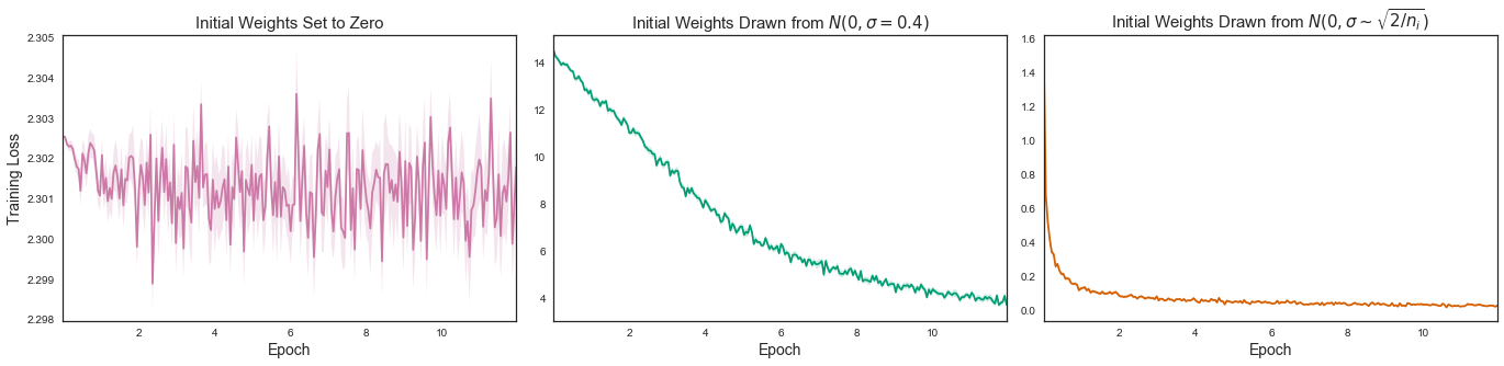\n\n We can also apply a Truncated Normal distribution using Keras, which will discard values more than 2 standard deviations from the mean. This could perhaps eliminate some outlier points during training."},{"metadata":{"trusted":true},"cell_type":"code","source":"weight_initializer = tf.keras.initializers.TruncatedNormal(stddev=weight_init_std, mean=weight_init_mean,\n seed=42)","execution_count":null,"outputs":[]},{"metadata":{},"cell_type":"markdown","source":"### Spectral Normalization"},{"metadata":{},"cell_type":"markdown","source":" Spectral Normalization is a new type of weight initialization, designed specifically for GANs, which seems to further stabilize model training (you can read more from this [paper](https://arxiv.org/pdf/1802.05957.pdf)). For a more detailed explanation on Spectral Normalization and why it works it also worth to check out this [post](https://christiancosgrove.com/blog/2018/01/04/spectral-normalization-explained.html), it has very intuitive examples.\n\n Spectral Normalization of a single weight in our network can be defined as the following:\n\n$$ \\sigma(W) = ||Wv|| = u^{T}Wv $$\n$$ W_{SN}(W) = \\frac{W}{\\sigma(W)} $$\n\n Here $u$ and $v$ are simple random vectors of the same size. They are utilized to perform what's called a power iteration operation on the specific weight, for each learning step and it proves to be a lot more computationally efficient than simply penalizing the gradients.\n\n Afterwards, in the backpropagation step, we use $W_{SN}(W)$ to update the weights instead of $W$.\n\n For this project, I will reuse some custom Keras layers implemented by IShengFang ([official code](https://github.com/IShengFang/SpectralNormalizationKeras)), to apply Spectral Normalization on top of Conv and Dense layers.\n\n Here is also a good example on the effect of Spectral Normalization:\n\nWith SN\n\n\nWithout SN\n"},{"metadata":{"trusted":true},"cell_type":"code","source":"class DenseSN(Dense):\n def build(self, input_shape):\n assert len(input_shape) >= 2\n input_dim = input_shape[-1]\n self.kernel = self.add_weight(shape=(input_dim, self.units),\n initializer=self.kernel_initializer,\n name='kernel',\n regularizer=self.kernel_regularizer,\n constraint=self.kernel_constraint)\n if self.use_bias:\n self.bias = self.add_weight(shape=(self.units,),\n initializer=self.bias_initializer,\n name='bias',\n regularizer=self.bias_regularizer,\n constraint=self.bias_constraint)\n else:\n self.bias = None\n self.u = self.add_weight(shape=tuple([1, self.kernel.shape.as_list()[-1]]),\n initializer=initializers.RandomNormal(0, 1),\n name='sn',\n trainable=False)\n self.input_spec = InputSpec(min_ndim=2, axes={-1: input_dim})\n self.built = True\n \n def call(self, inputs, training=None):\n def _l2normalize(v, eps=1e-12):\n return v / (K.sum(v ** 2) ** 0.5 + eps)\n def power_iteration(W, u):\n _u = u\n _v = _l2normalize(K.dot(_u, K.transpose(W)))\n _u = _l2normalize(K.dot(_v, W))\n return _u, _v\n W_shape = self.kernel.shape.as_list()\n #Flatten the Tensor\n W_reshaped = K.reshape(self.kernel, [-1, W_shape[-1]])\n _u, _v = power_iteration(W_reshaped, self.u)\n #Calculate Sigma\n sigma=K.dot(_v, W_reshaped)\n sigma=K.dot(sigma, K.transpose(_u))\n #normalize it\n W_bar = W_reshaped / sigma\n #reshape weight tensor\n if training in {0, False}:\n W_bar = K.reshape(W_bar, W_shape)\n else:\n with tf.control_dependencies([self.u.assign(_u)]):\n W_bar = K.reshape(W_bar, W_shape) \n output = K.dot(inputs, W_bar)\n if self.use_bias:\n output = K.bias_add(output, self.bias, data_format='channels_last')\n if self.activation is not None:\n output = self.activation(output)\n return output \n \nclass ConvSN2D(Conv2D):\n\n def build(self, input_shape):\n if self.data_format == 'channels_first':\n channel_axis = 1\n else:\n channel_axis = -1\n if input_shape[channel_axis] is None:\n raise ValueError('The channel dimension of the inputs '\n 'should be defined. Found `None`.')\n input_dim = input_shape[channel_axis]\n kernel_shape = self.kernel_size + (input_dim, self.filters)\n\n self.kernel = self.add_weight(shape=kernel_shape,\n initializer=self.kernel_initializer,\n name='kernel',\n regularizer=self.kernel_regularizer,\n constraint=self.kernel_constraint)\n\n if self.use_bias:\n self.bias = self.add_weight(shape=(self.filters,),\n initializer=self.bias_initializer,\n name='bias',\n regularizer=self.bias_regularizer,\n constraint=self.bias_constraint)\n else:\n self.bias = None\n \n self.u = self.add_weight(shape=tuple([1, self.kernel.shape.as_list()[-1]]),\n initializer=initializers.RandomNormal(0, 1),\n name='sn',\n trainable=False)\n \n # Set input spec.\n self.input_spec = InputSpec(ndim=self.rank + 2,\n axes={channel_axis: input_dim})\n self.built = True\n def call(self, inputs, training=None):\n def _l2normalize(v, eps=1e-12):\n return v / (K.sum(v ** 2) ** 0.5 + eps)\n def power_iteration(W, u):\n #Accroding the paper, we only need to do power iteration one time.\n _u = u\n _v = _l2normalize(K.dot(_u, K.transpose(W)))\n _u = _l2normalize(K.dot(_v, W))\n return _u, _v\n #Spectral Normalization\n W_shape = self.kernel.shape.as_list()\n #Flatten the Tensor\n W_reshaped = K.reshape(self.kernel, [-1, W_shape[-1]])\n _u, _v = power_iteration(W_reshaped, self.u)\n #Calculate Sigma\n sigma=K.dot(_v, W_reshaped)\n sigma=K.dot(sigma, K.transpose(_u))\n #normalize it\n W_bar = W_reshaped / sigma\n #reshape weight tensor\n if training in {0, False}:\n W_bar = K.reshape(W_bar, W_shape)\n else:\n with tf.control_dependencies([self.u.assign(_u)]):\n W_bar = K.reshape(W_bar, W_shape)\n \n outputs = K.conv2d(\n inputs,\n W_bar,\n strides=self.strides,\n padding=self.padding,\n data_format=self.data_format,\n dilation_rate=self.dilation_rate)\n if self.use_bias:\n outputs = K.bias_add(\n outputs,\n self.bias,\n data_format=self.data_format)\n if self.activation is not None:\n return self.activation(outputs)\n return outputs\n\nclass ConvSN2DTranspose(Conv2DTranspose):\n\n def build(self, input_shape):\n if len(input_shape) != 4:\n raise ValueError('Inputs should have rank ' +\n str(4) +\n '; Received input shape:', str(input_shape))\n if self.data_format == 'channels_first':\n channel_axis = 1\n else:\n channel_axis = -1\n if input_shape[channel_axis] is None:\n raise ValueError('The channel dimension of the inputs '\n 'should be defined. Found `None`.')\n input_dim = input_shape[channel_axis]\n kernel_shape = self.kernel_size + (self.filters, input_dim)\n\n self.kernel = self.add_weight(shape=kernel_shape,\n initializer=self.kernel_initializer,\n name='kernel',\n regularizer=self.kernel_regularizer,\n constraint=self.kernel_constraint)\n if self.use_bias:\n self.bias = self.add_weight(shape=(self.filters,),\n initializer=self.bias_initializer,\n name='bias',\n regularizer=self.bias_regularizer,\n constraint=self.bias_constraint)\n else:\n self.bias = None\n \n self.u = self.add_weight(shape=tuple([1, self.kernel.shape.as_list()[-1]]),\n initializer=initializers.RandomNormal(0, 1),\n name='sn',\n trainable=False)\n \n # Set input spec.\n self.input_spec = InputSpec(ndim=4, axes={channel_axis: input_dim})\n self.built = True \n \n def call(self, inputs):\n input_shape = K.shape(inputs)\n batch_size = input_shape[0]\n if self.data_format == 'channels_first':\n h_axis, w_axis = 2, 3\n else:\n h_axis, w_axis = 1, 2\n\n height, width = input_shape[h_axis], input_shape[w_axis]\n kernel_h, kernel_w = self.kernel_size\n stride_h, stride_w = self.strides\n if self.output_padding is None:\n out_pad_h = out_pad_w = None\n else:\n out_pad_h, out_pad_w = self.output_padding\n\n # Infer the dynamic output shape:\n out_height = conv_utils.deconv_length(height,\n stride_h, kernel_h,\n self.padding,\n out_pad_h)\n out_width = conv_utils.deconv_length(width,\n stride_w, kernel_w,\n self.padding,\n out_pad_w)\n if self.data_format == 'channels_first':\n output_shape = (batch_size, self.filters, out_height, out_width)\n else:\n output_shape = (batch_size, out_height, out_width, self.filters)\n \n #Spectral Normalization \n def _l2normalize(v, eps=1e-12):\n return v / (K.sum(v ** 2) ** 0.5 + eps)\n def power_iteration(W, u):\n #Accroding the paper, we only need to do power iteration one time.\n _u = u\n _v = _l2normalize(K.dot(_u, K.transpose(W)))\n _u = _l2normalize(K.dot(_v, W))\n return _u, _v\n W_shape = self.kernel.shape.as_list()\n #Flatten the Tensor\n W_reshaped = K.reshape(self.kernel, [-1, W_shape[-1]])\n _u, _v = power_iteration(W_reshaped, self.u)\n #Calculate Sigma\n sigma=K.dot(_v, W_reshaped)\n sigma=K.dot(sigma, K.transpose(_u))\n #normalize it\n W_bar = W_reshaped / sigma\n #reshape weight tensor\n if training in {0, False}:\n W_bar = K.reshape(W_bar, W_shape)\n else:\n with tf.control_dependencies([self.u.assign(_u)]):\n W_bar = K.reshape(W_bar, W_shape)\n self.kernel = W_bar\n \n outputs = K.conv2d_transpose(\n inputs,\n self.kernel,\n output_shape,\n self.strides,\n padding=self.padding,\n data_format=self.data_format)\n\n if self.use_bias:\n outputs = K.bias_add(\n outputs,\n self.bias,\n data_format=self.data_format)\n\n if self.activation is not None:\n return self.activation(outputs)\n return outputs","execution_count":null,"outputs":[]},{"metadata":{},"cell_type":"markdown","source":" Let's also define some template layers in Keras, so that we can create G and D more easily later on. The standard pattern for the layers will be:\n\nTP_Conv_Block = [(Conv(SN)2DTranspose (upsample)) -> (BatchNorm) -> (ReLU)]\n\nConv_Block = [(Conv(SN)2D (downsample)) -> (BatchNorm) -> (LeakyReLU)]"},{"metadata":{"trusted":true},"cell_type":"code","source":"def transposed_conv(model, out_channels, ksize, stride_size, ptype='same'):\n model.add(Conv2DTranspose(out_channels, (ksize, ksize),\n strides=(stride_size, stride_size), padding=ptype, \n kernel_initializer=weight_initializer, use_bias=False))\n model.add(BatchNormalization())\n model.add(ReLU())\n return model\n\ndef transposed_convSN(model, out_channels, ksize, stride_size, ptype='same'):\n model.add(ConvSN2DTranspose(out_channels, (ksize, ksize), \n strides=(stride_size, stride_size), padding=ptype, \n kernel_initializer=weight_initializer, use_bias=False))\n model.add(BatchNormalization())\n model.add(ReLU())\n return model\n\ndef convSN(model, out_channels, ksize, stride_size):\n model.add(ConvSN2D(out_channels, (ksize, ksize), strides=(stride_size, stride_size), padding='same',\n kernel_initializer=weight_initializer, use_bias=False))\n model.add(BatchNormalization())\n model.add(LeakyReLU(alpha=leaky_relu_slope))\n #model.add(Dropout(dropout_rate))\n return model\n\ndef conv(model, out_channels, ksize, stride_size):\n model.add(Conv2D(out_channels, (ksize, ksize), strides=(stride_size, stride_size), padding='same',\n kernel_initializer=weight_initializer, use_bias=False))\n model.add(BatchNormalization())\n model.add(LeakyReLU(alpha=leaky_relu_slope))\n #model.add(Dropout(dropout_rate))\n return model","execution_count":null,"outputs":[]},{"metadata":{},"cell_type":"markdown","source":"## The Generator"},{"metadata":{},"cell_type":"markdown","source":" We can finally define our generator. The model structure is mostly based on the official DCGAN [paper](https://arxiv.org/pdf/1511.06434.pdf) with a few tweaks that I found beneficial to the performance. Here is the overall structure:\n\n[Input(128, 1) -> Dense(2048,) -> Reshape(4, 4, 128) -> TP_Conv_Block(Depth=512, K=5x5, S=1x1) -> Dropout(0.5) -> TP_Conv_Block(Depth=256, K=5x5, S=2x2) -> Dropout(0.5) -> TP_Conv_Block(Depth=128, K=5x5, S=2x2) -> TP_Conv_Block(Depth=64, K=5x5, S=2x2) -> TP_Conv_Block(Depth=32, K=5x5, S=2x2) -> Dense(Depth=3, Tanh)]"},{"metadata":{"trusted":true},"cell_type":"code","source":"def DogGenerator():\n model = Sequential()\n model.add(Dense(image_width // scale_factor * image_height // scale_factor * 128,\n input_shape=(noise_dim,), kernel_initializer=weight_initializer))\n #model.add(BatchNormalization(epsilon=BN_EPSILON, momentum=BN_MOMENTUM))\n #model.add(LeakyReLU(alpha=leaky_relu_slope))\n model.add(Reshape((image_height // scale_factor, image_width // scale_factor, 128)))\n \n model = transposed_conv(model, 512, ksize=5, stride_size=1)\n model.add(Dropout(dropout_rate))\n model = transposed_conv(model, 256, ksize=5, stride_size=2)\n model.add(Dropout(dropout_rate))\n model = transposed_conv(model, 128, ksize=5, stride_size=2)\n model = transposed_conv(model, 64, ksize=5, stride_size=2)\n model = transposed_conv(model, 32, ksize=5, stride_size=2)\n \n model.add(Dense(3, activation='tanh', kernel_initializer=weight_initializer))\n\n return model","execution_count":null,"outputs":[]},{"metadata":{"trusted":true},"cell_type":"code","source":"dog_generator = DogGenerator()\nprint(dog_generator.summary())","execution_count":null,"outputs":[]},{"metadata":{},"cell_type":"markdown","source":" We can confirm that the Generator works initially by feeding it a random noise vector of the right size. The output image should be normalized to similar black-colored pixels due to the Weight Initialization step described earlier (they should be relatively zero-centered)."},{"metadata":{"trusted":true},"cell_type":"code","source":"# random noise vector\nnoise = tf.random.normal([1,noise_dim])\n#sample = generate_latent_points(100, 50)\n# run the generator model with the noise vector as input\ngenerated_image = dog_generator(noise, training=False)\n# display output\nplt.imshow(generated_image[0, :, :, :])\nprint(generated_image.shape)\n#print(sample.shape, sample.mean(), sample.std())\nprint(noise.shape, tf.math.reduce_mean(noise).numpy(), tf.math.reduce_std(noise).numpy())","execution_count":null,"outputs":[]},{"metadata":{},"cell_type":"markdown","source":"## The Discriminator"},{"metadata":{},"cell_type":"markdown","source":" The Discriminator is relatively easier to implement, since its basically a small CNN two-class classifier. We can choose whether to apply Spectral Normalization or not and see the performance effects. For this example, I will try to apply SN only in D. Here is D's structure:\n\n[Input(128, 128, 3) -> Conv(SN)2D(Depth=64, K=5x5, S=1x1, same) -> LeakyReLU -> Conv_Block(Depth=64, K=5x5, S=2x2) -> Conv_Block(Depth=128, K=5x5, S=2x2) -> Conv_Block(Depth=256, K=5x5, S=2x2) -> Flatten -> Dense(16384, Sigmoid)]\n\n \n Also note that all Conv and Dense layers are initialized with the Truncated Normal distribution defined above. Another thing is that the bias term is removed from the Conv layers, which also stabilizes the model a little bit."},{"metadata":{"trusted":true},"cell_type":"code","source":"def DogDiscriminator(spectral_normalization=True):\n model = Sequential()\n if spectral_normalization:\n model.add(ConvSN2D(64, (5, 5), strides=(1,1), padding='same', use_bias=False,\n input_shape=[image_height, image_width, image_channels], \n kernel_initializer=weight_initializer))\n #model.add(BatchNormalization(epsilon=BN_EPSILON, momentum=BN_MOMENTUM))\n model.add(LeakyReLU(alpha=leaky_relu_slope))\n #model.add(Dropout(dropout_rate))\n \n model = convSN(model, 64, ksize=5, stride_size=2)\n #model = convSN(model, 128, ksize=3, stride_size=1)\n model = convSN(model, 128, ksize=5, stride_size=2)\n #model = convSN(model, 256, ksize=3, stride_size=1)\n model = convSN(model, 256, ksize=5, stride_size=2)\n #model = convSN(model, 512, ksize=3, stride_size=1)\n #model.add(Dropout(dropout_rate))\n\n model.add(Flatten())\n model.add(DenseSN(1, activation='sigmoid'))\n else:\n model.add(Conv2D(64, (4, 4), strides=(2,2), padding='same', use_bias=False,\n input_shape=[image_height, image_width, image_channels], \n kernel_initializer=weight_initializer))\n #model.add(BatchNormalization(epsilon=BN_EPSILON, momentum=BN_MOMENTUM))\n model.add(LeakyReLU(alpha=leaky_relu_slope))\n #model.add(Dropout(dropout_rate))\n\n model = conv(model, 64, ksize=4, stride_size=2)\n #model = convSN(model, 128, ksize=3, stride_size=1)\n model = conv(model, 128, ksize=4, stride_size=2)\n #model = convSN(model, 256, ksize=3, stride_size=1)\n model = conv(model, 256, ksize=4, stride_size=2)\n #model = convSN(model, 512, ksize=3, stride_size=1)\n\n model.add(Flatten())\n model.add(Dense(1, activation='sigmoid'))\n return model","execution_count":null,"outputs":[]},{"metadata":{"trusted":true},"cell_type":"code","source":"dog_discriminator = DogDiscriminator(spectral_normalization=True)\nprint(dog_discriminator.summary())","execution_count":null,"outputs":[]},{"metadata":{},"cell_type":"markdown","source":"Below we can observe, that D indeed outputs a probability very close to 0.5 for a noisy input."},{"metadata":{"trusted":true},"cell_type":"code","source":"decision = dog_discriminator(generated_image)\nprint(decision)","execution_count":null,"outputs":[]},{"metadata":{},"cell_type":"markdown","source":"## Further optimization tricks"},{"metadata":{},"cell_type":"markdown","source":"### Label smoothing"},{"metadata":{},"cell_type":"markdown","source":" One regularization method that can be applied during training is called Label smoothing. What this does is that it essentially prevents D from being overconfident or underconfident in its predictions. If D becomes too certain that there is a dog in a specific image, G can exploit that fact and continuously start to generate only images of that sort and in turn, cease to improve. We can combat this, by setting the class labels to be in the range [0, 0.3] for the negative classes and [0.7, 1] for the positive ones. \n\n This will prevent the overall probabilities from getting very close to the two thresholds."},{"metadata":{"trusted":true},"cell_type":"code","source":"# Label smoothing -- technique from GAN hacks, instead of assigning 1/0 as class labels, we assign a random integer in range [0.7, 1.0] for positive class\n# and [0.0, 0.3] for negative class\n\ndef smooth_positive_labels(y):\n return y - 0.3 + (np.random.random(y.shape) * 0.5)\n\ndef smooth_negative_labels(y):\n return y + np.random.random(y.shape) * 0.3","execution_count":null,"outputs":[]},{"metadata":{},"cell_type":"markdown","source":"### Introducing some noise to the labels"},{"metadata":{},"cell_type":"markdown","source":" This technique is also called Instance Noise. By adding a small amount of error to the labels (let's say 5%), this tends to make the true and predicted distributions more spread out and thus start to overlap with each other. This in turn makes fitting a custom distribution of generated images easier in the learning process.\n\n Here is a good example of how the two distributions look like with these techniques:\n\n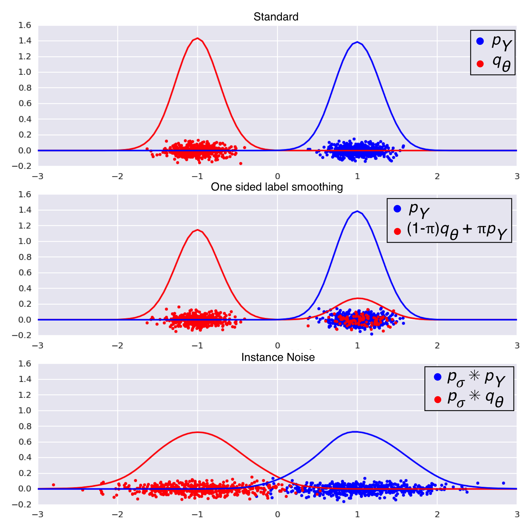"},{"metadata":{"trusted":true},"cell_type":"code","source":"# randomly flip some labels\ndef noisy_labels(y, p_flip):\n # determine the number of labels to flip\n n_select = int(p_flip * int(y.shape[0]))\n # choose labels to flip\n flip_ix = np.random.choice([i for i in range(int(y.shape[0]))], size=n_select)\n \n op_list = []\n # invert the labels in place\n #y_np[flip_ix] = 1 - y_np[flip_ix]\n for i in range(int(y.shape[0])):\n if i in flip_ix:\n op_list.append(tf.subtract(1, y[i]))\n else:\n op_list.append(y[i])\n \n outputs = tf.stack(op_list)\n return outputs","execution_count":null,"outputs":[]},{"metadata":{},"cell_type":"markdown","source":"### Optimizers"},{"metadata":{},"cell_type":"markdown","source":" The best proven optimization algorithm for this task is Adam with a standard learning rate of 0.0002 for both models and a beta of 0.5."},{"metadata":{"trusted":true},"cell_type":"code","source":"generator_optimizer = tf.train.AdamOptimizer(learning_rate=lr_initial_g, beta1=0.5)\ndiscriminator_optimizer = tf.train.AdamOptimizer(learning_rate=lr_initial_d, beta1=0.5)\n# This method returns a helper function to compute cross entropy loss\ncross_entropy = tf.keras.losses.BinaryCrossentropy(from_logits=False)","execution_count":null,"outputs":[]},{"metadata":{},"cell_type":"markdown","source":"### Defining the loss functions"},{"metadata":{},"cell_type":"markdown","source":" Another new trend in optimizing GANs recently has been applying a Relativistic loss function as opposed to the standard one. Those functions measure the probability that the real data is more \"realistic\" than the generated data. One of the more popular relativistic function choices include RaLSGAN (Relativistic Average Least Squares), RaSGAN (Relativistic Average Standard) and RaHinge (Relativistic Hinge loss).\n\n But before all of that, let's define the standard GAN loss:\n\n$$ \\underset{D}{min}(V(D)) = - E_{x}[\\log{D(x)}] - E_{z}[\\log{(1-D(G(z)))}] $$\n\n As we can observe, this is basically the standard Binary Crossentropy loss used for classification tasks or the Logistic Loss between the real and generated distributions.\n\n In comparison, here is what an RSGAN (Relativistic Standard) loss looks like:\n\n$$ L^{RSGAN}_{D} = - E_{(x_{r},x_{f})}[\\log{(sigmoid(C(x_{r}) - C(x_{f})))}] $$\n$$ L^{RSGAN}_{G} = - E_{(x_{r},x_{f})}[\\log{(sigmoid(C(x_{f}) - C(x_{r})))}] $$\n\n In this case the task is different, to measure the similarity between the real (r) and fake (f) data distributions. RSGAN reaches the optimal point when D(x) = 0.5 (i.e. $C(x_{r}) = C(x_{f})$). There are many relativistic loss function variants and they all contain different methods for measuring this similarity. In this project, I've tried out 3 of the variants that seemed to have the best documented MIFID score (RaLSGAN, RaSGAN and RaHinge). Feel free to try out different losses for yourself to see if you can improve the performance ;). Here's a big list of the most commonly used ones:\n\n"},{"metadata":{},"cell_type":"markdown","source":" With this in mind, I have devised a nice little decision tree function for choosing the losses for both G and D. Note that instance noise and label smoothing need to be applied before calculating the actual losses. \n\n Throughout many trials for this particular problem, I didn't find any increase in performance by switching to Relativistic losses, so I decided to stick with the standard GAN loss function, as it is much simpler to estimate, though in some cases these losses can really speed up convergence in your model."},{"metadata":{"trusted":true},"cell_type":"code","source":"def discriminator_loss(real_output, fake_output, loss_func, apply_label_smoothing=True, label_noise=True):\n if label_noise and apply_label_smoothing:\n real_output_noise = noisy_labels(tf.ones_like(real_output), 0.05)\n fake_output_noise = noisy_labels(tf.zeros_like(fake_output), 0.05)\n real_output_smooth = smooth_positive_labels(real_output_noise)\n fake_output_smooth = smooth_negative_labels(fake_output_noise)\n if loss_func == 'gan': \n real_loss = cross_entropy(tf.ones_like(real_output_smooth), real_output)\n fake_loss = cross_entropy(tf.zeros_like(fake_output_smooth), fake_output)\n else:\n if loss_func == 'ralsgan':\n return (tf.reduce_mean(tf.square(real_output_smooth - tf.reduce_mean(fake_output_smooth) - tf.ones_like(real_output_smooth)))\n + tf.reduce_mean(tf.square(fake_output_smooth - tf.reduce_mean(real_output_smooth) + tf.ones_like(fake_output_smooth)))) / 2.\n elif loss_func == 'rasgan':\n avg_fake_logit = tf.reduce_mean(fake_output_smooth)\n avg_real_logit = tf.reduce_mean(real_output_smooth)\n D_r_tilde = tf.nn.sigmoid(real_output_smooth - avg_fake_logit)\n D_f_tilde = tf.nn.sigmoid(fake_output_smooth - avg_real_logit)\n total_loss = - tf.reduce_mean(tf.log(\n D_r_tilde + 1e-14)) - tf.reduce_mean(tf.log(1 - D_f_tilde + 1e-14))\n return total_loss\n elif loss_func == 'rahinge':\n real_loss = tf.reduce_mean(tf.nn.relu(tf.ones_like(real_output_smooth) - (real_output_smooth - tf.reduce_mean(fake_output_smooth))))\n fake_loss = tf.reduce_mean(tf.nn.relu(tf.ones_like(fake_output_smooth) + (fake_output_smooth - tf.reduce_mean(real_output_smooth))))\n total_loss = real_loss + fake_loss\n return total_loss\n elif label_noise and not apply_label_smoothing:\n real_output_noise = noisy_labels(tf.ones_like(real_output), 0.05)\n fake_output_noise = noisy_labels(tf.zeros_like(fake_output), 0.05)\n if loss_func == 'gan': \n real_loss = cross_entropy(tf.ones_like(real_output_noise), real_output)\n fake_loss = cross_entropy(tf.zeros_like(fake_output_noise), fake_output)\n else:\n if loss_func == 'ralsgan':\n return (tf.reduce_mean(tf.square(real_output_noise - tf.reduce_mean(fake_output_noise) - tf.ones_like(real_output_noise)))\n + tf.reduce_mean(tf.square(fake_output_noise - tf.reduce_mean(real_output_noise) + tf.ones_like(fake_output_noise)))) / 2.\n elif loss_func == 'rasgan':\n avg_fake_logit = tf.reduce_mean(fake_output_noise)\n avg_real_logit = tf.reduce_mean(real_output_noise)\n D_r_tilde = tf.nn.sigmoid(real_output_noise - avg_fake_logit)\n D_f_tilde = tf.nn.sigmoid(fake_output_noise - avg_real_logit)\n total_loss = - tf.reduce_mean(tf.log(\n D_r_tilde + 1e-14)) - tf.reduce_mean(tf.log(1 - D_f_tilde + 1e-14))\n return total_loss\n elif loss_func == 'rahinge':\n real_loss = tf.reduce_mean(tf.nn.relu(tf.ones_like(real_output_noise) - (real_output_noise - tf.reduce_mean(fake_output_noise))))\n fake_loss = tf.reduce_mean(tf.nn.relu(tf.ones_like(fake_output_noise) + (fake_output_noise - tf.reduce_mean(real_output_noise))))\n total_loss = real_loss + fake_loss\n return total_loss\n elif apply_label_smoothing and not label_noise:\n real_output_smooth = smooth_positive_labels(tf.ones_like(real_output))\n fake_output_smooth = smooth_negative_labels(tf.zeros_like(fake_output))\n if loss_func == 'gan': \n real_loss = cross_entropy(tf.ones_like(real_output_smooth), real_output)\n fake_loss = cross_entropy(tf.zeros_like(fake_output_smooth), fake_output)\n else:\n if loss_func == 'ralsgan':\n return (tf.reduce_mean(tf.square(real_output_smooth - tf.reduce_mean(fake_output_smooth) - tf.ones_like(real_output_smooth)))\n + tf.reduce_mean(tf.square(fake_output_smooth - tf.reduce_mean(real_output_smooth) + tf.ones_like(fake_output_smooth)))) / 2.\n elif loss_func == 'rasgan':\n avg_fake_logit = tf.reduce_mean(fake_output_smooth)\n avg_real_logit = tf.reduce_mean(real_output_smooth)\n D_r_tilde = tf.nn.sigmoid(real_output_smooth - avg_fake_logit)\n D_f_tilde = tf.nn.sigmoid(fake_output_smooth - avg_real_logit)\n total_loss = - tf.reduce_mean(tf.log(\n D_r_tilde + 1e-14)) - tf.reduce_mean(tf.log(1 - D_f_tilde + 1e-14))\n return total_loss\n elif loss_func == 'rahinge':\n real_loss = tf.reduce_mean(tf.nn.relu(tf.ones_like(real_output_smooth) - (real_output_smooth - tf.reduce_mean(fake_output_smooth))))\n fake_loss = tf.reduce_mean(tf.nn.relu(tf.ones_like(fake_output_smooth) + (fake_output_smooth - tf.reduce_mean(real_output_smooth))))\n total_loss = real_loss + fake_loss\n return total_loss \n else:\n if loss_func == 'gan': \n real_loss = cross_entropy(tf.ones_like(real_output), real_output)\n fake_loss = cross_entropy(tf.zeros_like(fake_output), fake_output)\n else:\n if loss_func == 'ralsgan':\n return (tf.reduce_mean(tf.square(real_output - tf.reduce_mean(fake_output) - tf.ones_like(real_output)))\n + tf.reduce_mean(tf.square(fake_output - tf.reduce_mean(real_output) + tf.ones_like(fake_output)))) / 2.\n elif loss_func == 'rasgan':\n avg_fake_logit = tf.reduce_mean(fake_output)\n avg_real_logit = tf.reduce_mean(real_output)\n D_r_tilde = tf.nn.sigmoid(real_output - avg_fake_logit)\n D_f_tilde = tf.nn.sigmoid(fake_output - avg_real_logit)\n total_loss = - tf.reduce_mean(tf.log(\n D_r_tilde + 1e-14)) - tf.reduce_mean(tf.log(1 - D_f_tilde + 1e-14))\n return total_loss\n elif loss_func == 'rahinge':\n real_loss = tf.reduce_mean(tf.nn.relu(tf.ones_like(real_output) - (real_output - tf.reduce_mean(fake_output))))\n fake_loss = tf.reduce_mean(tf.nn.relu(tf.ones_like(fake_output) + (fake_output - tf.reduce_mean(real_output))))\n total_loss = real_loss + fake_loss\n return total_loss","execution_count":null,"outputs":[]},{"metadata":{"trusted":true},"cell_type":"code","source":"def generator_loss(real_output, fake_output, loss_func, apply_label_smoothing=True):\n if apply_label_smoothing:\n fake_output_smooth = smooth_negative_labels(tf.ones_like(fake_output))\n if loss_func == 'gan':\n return cross_entropy(tf.ones_like(fake_output_smooth), fake_output)\n else:\n if loss_func == 'ralsgan':\n return (tf.reduce_mean(tf.square(real_output - tf.reduce_mean(fake_output_smooth) + tf.ones_like(real_output)))\n + tf.reduce_mean(tf.square(fake_output_smooth - tf.reduce_mean(real_output) - tf.ones_like(fake_output_smooth)))) / 2.\n elif loss_func == 'rasgan':\n avg_fake_logit = tf.reduce_mean(fake_output_smooth)\n avg_real_logit = tf.reduce_mean(real_output)\n D_r_tilde = tf.nn.sigmoid(real_output - avg_fake_logit)\n D_f_tilde = tf.nn.sigmoid(fake_output_smooth - avg_real_logit)\n total_loss = - tf.reduce_mean(tf.log(\n D_f_tilde + 1e-14)) - tf.reduce_mean(tf.log(1 - D_r_tilde + 1e-14))\n return total_loss\n elif loss_func == 'rahinge':\n fake_loss = tf.reduce_mean(tf.nn.relu(tf.ones_like(fake_output_smooth) - (fake_output_smooth - tf.reduce_mean(real_output))))\n real_loss = tf.reduce_mean(tf.nn.relu(tf.ones_like(real_output) + (real_output - tf.reduce_mean(fake_output_smooth))))\n loss = fake_loss + real_loss\n return loss\n else: \n if loss_func == 'gan':\n return cross_entropy(tf.ones_like(fake_output), fake_output)\n else:\n if loss_func == 'ralsgan':\n return (tf.reduce_mean(tf.square(real_output - tf.reduce_mean(fake_output) + tf.ones_like(real_output)))\n + tf.reduce_mean(tf.square(fake_output - tf.reduce_mean(real_output) - tf.ones_like(fake_output)))) / 2.\n elif loss_func == 'rasgan':\n avg_fake_logit = tf.reduce_mean(fake_output)\n avg_real_logit = tf.reduce_mean(real_output)\n D_r_tilde = tf.nn.sigmoid(real_output - avg_fake_logit)\n D_f_tilde = tf.nn.sigmoid(fake_output - avg_real_logit)\n total_loss = - tf.reduce_mean(tf.log(\n D_f_tilde + 1e-14)) - tf.reduce_mean(tf.log(1 - D_r_tilde + 1e-14))\n return total_loss\n elif loss_func == 'rahinge':\n fake_loss = tf.reduce_mean(tf.nn.relu(tf.ones_like(fake_output) - (fake_output - tf.reduce_mean(real_output))))\n real_loss = tf.reduce_mean(tf.nn.relu(tf.ones_like(real_output) + (real_output - tf.reduce_mean(fake_output))))\n loss = fake_loss + real_loss\n return loss ","execution_count":null,"outputs":[]},{"metadata":{},"cell_type":"markdown","source":"### Define a checkpointer"},{"metadata":{},"cell_type":"markdown","source":" Let's finally add a checkpointer to be able to save and reuse our model."},{"metadata":{"trusted":true},"cell_type":"code","source":"checkpoint_dir = '/training_checkpoints'\ncheckpoint_prefix = os.path.join(checkpoint_dir, \"ckpt\")\ncheckpoint = tf.train.Checkpoint(generator_optimizer=generator_optimizer,\n discriminator_optimizer=discriminator_optimizer,\n generator=dog_generator,\n discriminator=dog_discriminator)","execution_count":null,"outputs":[]},{"metadata":{},"cell_type":"markdown","source":"### Main training loop"},{"metadata":{},"cell_type":"markdown","source":" Let's also fix the number of epochs for training and the number of images to feed to the Generator for visualizing results during that training."},{"metadata":{"trusted":true},"cell_type":"code","source":"EPOCHS = 280\nnum_examples_to_generate = 64\nseed = tf.random.normal([num_examples_to_generate, noise_dim])","execution_count":null,"outputs":[]},{"metadata":{},"cell_type":"markdown","source":" One training step of a DCGAN consists of three standard steps:\n\n1. Forward prop - G creates a batch of fake images; this, alongside a batch of real images is fed to D.\n2. Calculate both G and D's loss function.\n3. Backprop - compute gradients for G and D optimize the weights."},{"metadata":{"trusted":true},"cell_type":"code","source":"def train_step(images, loss_type='gan'):\n noise = tf.random.normal([batch_size, noise_dim])\n\n with tf.GradientTape() as gen_tape, tf.GradientTape() as disc_tape:\n generated_images = dog_generator(noise, training=True)\n \n real_output = dog_discriminator(images, training=True)\n fake_output = dog_discriminator(generated_images, training=True)\n \n gen_loss = generator_loss(real_output, fake_output, loss_type, apply_label_smoothing=True)\n disc_loss = discriminator_loss(real_output, fake_output, loss_type, \n apply_label_smoothing=True, label_noise=True)\n \n gradients_of_generator = gen_tape.gradient(gen_loss, dog_generator.trainable_variables)\n gradients_of_discriminator = disc_tape.gradient(disc_loss, dog_discriminator.trainable_variables)\n\n generator_optimizer.apply_gradients(zip(gradients_of_generator, dog_generator.trainable_variables))\n discriminator_optimizer.apply_gradients(zip(gradients_of_discriminator, dog_discriminator.trainable_variables))\n \n return gen_loss, disc_loss","execution_count":null,"outputs":[]},{"metadata":{},"cell_type":"markdown","source":" Let's also define some functions to visualize the model losses by epoch and as a whole."},{"metadata":{"trusted":true},"cell_type":"code","source":"def plot_losses(G_losses, D_losses, all_gl, all_dl, epoch):\n plt.figure(figsize=(10,5))\n plt.title(\"Generator and Discriminator Loss - EPOCH {}\".format(epoch))\n plt.plot(G_losses,label=\"G\")\n plt.plot(D_losses,label=\"D\")\n plt.xlabel(\"Iterations\")\n plt.ylabel(\"Loss\")\n plt.legend()\n ymax = plt.ylim()[1]\n plt.show()\n \n plt.figure(figsize=(10,5))\n plt.plot(np.arange(len(all_gl)),all_gl,label='G')\n plt.plot(np.arange(len(all_dl)),all_dl,label='D')\n plt.legend()\n #plt.ylim((0,np.min([1.1*np.max(all_gl),2*ymax])))\n plt.title('All Time Loss')\n plt.show()","execution_count":null,"outputs":[]},{"metadata":{},"cell_type":"markdown","source":" We can also use the following function to plot a grid of the generated images."},{"metadata":{"trusted":true},"cell_type":"code","source":"def generate_and_save_images(model, epoch, test_input, rows, cols):\n # Notice `training` is set to False.\n # This is so all layers run in inference mode (batchnorm).\n predictions = model(test_input, training=False)\n fig = plt.figure(figsize=(14,14))\n for i in range(predictions.shape[0]):\n plt.subplot(rows, cols, i+1)\n plt.imshow((predictions[i, :, :, :] * 127.5 + 127.5) / 255.)\n plt.axis('off') \n \n plt.subplots_adjust(wspace=0, hspace=0)\n plt.savefig('image_at_epoch_{:04d}.png'.format(epoch))\n plt.show()","execution_count":null,"outputs":[]},{"metadata":{},"cell_type":"markdown","source":" To generate a single test image, we can also reuse the same method."},{"metadata":{"trusted":true},"cell_type":"code","source":"def generate_test_image(model, noise_dim=noise_dim):\n test_input = tf.random.normal([1, noise_dim])\n # Notice `training` is set to False.\n # This is so all layers run in inference mode (batchnorm).\n predictions = model(test_input, training=False)\n fig = plt.figure(figsize=(5,5))\n plt.imshow((predictions[0, :, :, :] * 127.5 + 127.5) / 255.)\n plt.axis('off') \n plt.show()","execution_count":null,"outputs":[]},{"metadata":{},"cell_type":"markdown","source":"## Evaluating GANs - FID and MIFID"},{"metadata":{},"cell_type":"markdown","source":"### Inception Score"},{"metadata":{},"cell_type":"markdown","source":" We still haven't mentioned how a GAN is usually evaluated. Most research papers that use benchmarks to estimate how well a GAN performs are usually based on what's called the Inception Score. This measures two main characteristics of the input images:\n\n- The variety (for example generating different types of dog breeds)\n- The distinction (or quality of the image)\n\n If both things are true, the score will be high. If either or both are false, the score will be low.\nA higher score is better. It means your GAN can generate many different distinct images. The lowest score possible is zero. Mathematically the highest possible score is infinity, although in practice there will probably emerge a non-infinite ceiling.\n\n The Inception Score is derived from Google's [Inception Network](https://towardsdatascience.com/a-simple-guide-to-the-versions-of-the-inception-network-7fc52b863202), which is one of the state-of-the-art deep architectures for classifying images. By passing the images from our GAN through the classifier, we can measure properties of our generated images. To produce the score, we need to calculate the similarity/distance between the real and fake distributions of images. This is done using the KL(Kullback–Leibler) divergence formula: \n\n$$ D_{KL}(P \\:||\\:Q) = - \\sum_{x \\in X}P(x)\\log{\\frac{Q(x)}{P(x)}} $$\n\n Here, P and Q are the two measured distributions. In this case, higher KL divergence means better results - the quality of the images is similar and there is a wide variety of labels present. In the opposite case, the low KL divergence can be due to either low quality or low variety of labels:\n\n"},{"metadata":{},"cell_type":"markdown","source":"### FID (Frechet Inception Distance)"},{"metadata":{},"cell_type":"markdown","source":" One shortcoming for IS is that it can misrepresent the performance if it only generates one image per class. To combat this we can use the FID (Frechet Inception Distance). This measure defines the two previous types of images as multivariate Gaussian distributions with mean $\\mu$ and covariance $\\Sigma$ (Sigma). Let's see how this distance is calculated:\n\n$$ FID(x,\\:g) = \\big\\|\\mu_{x} - \\mu_{g}\\big\\|^2_2 + Tr(\\Sigma_{x} + \\Sigma_{g} - 2(\\Sigma_{x}\\Sigma_{g})^{\\frac{1}{2}}) $$\n\n Here, $x$ and $g$ represent the real and fake distribution of images, while $Tr$ is the sum of diagonal elements of the results.\n\n> Lower FID values mean better image quality and diversity. \n\n"},{"metadata":{},"cell_type":"markdown","source":" Here are also a few useful notes on why FID is a good measure:\n\n> - FID is more robust to noise than IS.\n> - If the model only generates one image per class, the distance will be high. So FID is a better measurement for image diversity.\n> - By computing the FID between a training dataset and a testing dataset, we should expect the FID to be zero since both are real images. (although there is usually a small amount of error)\n> - FID and IS are based on feature extraction (the presence or the absence of features)."},{"metadata":{},"cell_type":"markdown","source":"### MIFID (Memorization Informed Frechet Inception Distance)"},{"metadata":{},"cell_type":"markdown","source":" Here is Kaggle's official evaluation workflow for this competition:\n\n"},{"metadata":{},"cell_type":"markdown","source":" As we can see, in addition to the FID metric, there is an additional Memorization Score added to the calculation. This is basically a Cosine distance formula that measures the similarity between the real and fake images. My guess is that this has been done to make sure that the images fed to the evaluation kernel have actually been generated by a GAN and not just replicated or modified from the real dataset.\n\n Thankfully, the MIFID evaluator has been implemented by the Kaggle team [(here)](https://www.kaggle.com/wendykan/demo-mifid-metric-for-dog-image-generation-comp) and we don't have to worry about it. \nTo use it, make sure you add this [dataset](https://www.kaggle.com/wendykan/dog-face-generation-competition-kid-metric-input) to your input."},{"metadata":{"trusted":true},"cell_type":"code","source":"class KernelEvalException(Exception):\n pass\n\n\n@dataclass\nclass MiFIDEvaluator(object):\n model_path: str\n train_images_path: str\n feature_path: str = None\n imsize: int = 64\n output_layer: str = 'Pretrained_Net/pool_3:0'\n input_layer: str = 'Pretrained_Net/ExpandDims:0'\n output_shape: int = 2048\n cosine_distance_eps: float = 0.1\n batch_size: int = 50\n fid_epsilon: float = 1e-14\n \n def __post_init__(self):\n tf.reset_default_graph()\n self.create_model_graph()\n with tf.Session() as sess:\n if self.feature_path is None:\n self.mu2, self.sigma2, self.features2 = self._handle_path_memorization(\n self.train_images_path, sess, is_checksize=False, is_check_png=False)\n else:\n with np.load(self.feature_path) as f:\n self.mu2, self.sigma2, self.features2 = f['m'], f['s'], f['features']\n \n def create_model_graph(self):\n with tf.gfile.FastGFile(self.model_path, 'rb') as f:\n graph_def = tf.GraphDef()\n graph_def.ParseFromString(f.read())\n _ = tf.import_graph_def(graph_def, name='Pretrained_Net')\n \n def img_read_checks(self, filename, is_checksize=False, is_check_png=False):\n im = Image.open(str(filename))\n if is_checksize and im.size != (self.imsize, self.imsize):\n raise KernelEvalException(f'The images are not of size {check_imsize}')\n if is_check_png and im.format != 'PNG':\n raise KernelEvalException('Only PNG images should be submitted.')\n\n if self.imsize is None:\n return im\n else:\n return im.resize((self.imsize, self.imsize), Image.ANTIALIAS)\n \n def _get_model_layer(self, sess):\n layer = sess.graph.get_tensor_by_name(self.output_layer)\n ops = layer.graph.get_operations()\n for op_idx, op in enumerate(ops):\n for o in op.outputs:\n shape = o.get_shape()\n if shape._dims != []:\n shape = [s.value for s in shape]\n new_shape = []\n for j, s in enumerate(shape):\n if s == 1 and j == 0:\n new_shape.append(None)\n else:\n new_shape.append(s)\n o.__dict__['_shape_val'] = tf.TensorShape(new_shape)\n return layer\n \n def get_activations(self, images, sess):\n inception_layer = self._get_model_layer(sess)\n n_images = images.shape[0]\n if self.batch_size > n_images:\n warnings.warn('batch size is bigger than the data size. setting batch size to data size')\n self.batch_size = n_images\n n_batches = n_images // self.batch_size + 1\n pred_arr = np.empty((n_images, self.output_shape))\n for i in range(n_batches):\n start = i * self.batch_size\n if start + self.batch_size < n_images:\n end = start + self.batch_size\n else:\n end = n_images\n\n batch = images[start:end]\n pred = sess.run(inception_layer, {self.input_layer: batch})\n pred_arr[start:end] = pred.reshape(-1, self.output_shape)\n return pred_arr\n \n def calculate_activation_statistics(self, images, sess):\n act = self.get_activations(images, sess)\n mu = np.mean(act, axis=0)\n sigma = np.cov(act, rowvar=False)\n return mu, sigma, act\n \n def _handle_path_memorization(self, path, sess, is_checksize, is_check_png):\n path = Path(path)\n files = list(path.glob('*.jpg')) + list(path.glob('*.png'))\n\n # In production we don't resize input images. This is just for demo purpose. \n x = np.array([np.array(self.img_read_checks(fn, is_checksize, is_check_png)) for fn in files])\n m, s, features = self.calculate_activation_statistics(x, sess)\n del x\n return m, s, features\n \n def calculate_frechet_distance(self, mu1, sigma1):\n mu1 = np.atleast_1d(mu1)\n mu2 = np.atleast_1d(self.mu2)\n sigma1 = np.atleast_2d(sigma1)\n sigma2 = np.atleast_2d(self.sigma2)\n\n assert mu1.shape == mu2.shape, 'Training and test mean vectors have different lengths'\n assert sigma1.shape == sigma2.shape, 'Training and test covariances have different dimensions'\n\n # product might be almost singular\n covmean, _ = linalg.sqrtm(sigma1.dot(sigma2), disp=False)\n if not np.isfinite(covmean).all():\n msg = f'fid calculation produces singular product; adding {self.eps} to diagonal of cov estimates'\n warnings.warn(msg)\n offset = np.eye(sigma1.shape[0]) * self.eps\n covmean = linalg.sqrtm((sigma1 + offset).dot(sigma2 + offset))\n \n # numerical error might give slight imaginary component\n if np.iscomplexobj(covmean):\n if not np.allclose(np.diagonal(covmean).imag, 0, atol=1e-3):\n m = np.max(np.abs(covmean.imag))\n raise ValueError(f'Imaginary component {m}')\n covmean = covmean.real\n tr_covmean = np.trace(covmean)\n return (mu1 - mu2).dot(mu1 - mu2) + np.trace(sigma1) + np.trace(sigma2) - 2 * tr_covmean\n \n @staticmethod\n def normalize_rows(x):\n return np.nan_to_num(x / np.linalg.norm(x, ord=2, axis=1, keepdims=True))\n \n def cosine_distance(self, features1):\n features1_nozero = features1[np.sum(features1, axis=1) != 0]\n features2_nozero = self.features2[np.sum(self.features2, axis=1) != 0]\n norm_f1 = self.normalize_rows(features1_nozero)\n norm_f2 = self.normalize_rows(features2_nozero)\n\n d = 1.0 - np.abs(np.matmul(norm_f1, norm_f2.T))\n mean_min_d = np.mean(np.min(d, axis=1))\n return mean_min_d\n \n def calculate_kid_given_paths(self, user_images_unzipped_path):\n with tf.Session() as sess:\n sess.run(tf.global_variables_initializer())\n m1, s1, features1 = self._handle_path_memorization(\n user_images_unzipped_path, sess, is_checksize=True, is_check_png=True)\n\n fid_value = self.calculate_frechet_distance(m1, s1)\n distance = self.cosine_distance(features1)\n return fid_value, distance\n \n def distance_thresholding(self, d):\n if d < self.cosine_distance_eps:\n return d\n else:\n return 1\n \n def evaluate(self, user_images_unzipped_path):\n fid_value, distance = self.calculate_kid_given_paths(user_images_unzipped_path)\n distance = self.distance_thresholding(distance)\n return fid_value, distance, fid_value / (distance + self.fid_epsilon)","execution_count":null,"outputs":[]},{"metadata":{},"cell_type":"markdown","source":"### Image zipping and saving functions"},{"metadata":{},"cell_type":"markdown","source":" I'm just going to add two more for zipping the final 10K images for submission and generating temporary images to calculate the MIFID in between certain epochs during training."},{"metadata":{"trusted":true},"cell_type":"code","source":"def zip_images(filename='images.zip'):\n # SAVE TO ZIP FILE NAMED IMAGES.ZIP\n z = zipfile.PyZipFile(filename, mode='w')\n for k in range(image_sample_size):\n generated_image = dog_generator(tf.random.normal([1, noise_dim]), training=False)\n f = str(k)+'.png'\n img = np.array(generated_image)\n img = (img[0, :, :, :] + 1.) / 2.\n img = Image.fromarray((255*img).astype('uint8').reshape((image_height,image_width,image_channels)))\n img.save(f,'PNG')\n z.write(f)\n os.remove(f)\n #if k % 1000==0: print(k)\n z.close()\n print('Saved final images for submission.')\n \ndef save_images(directory=OUT_DIR):\n for k in range(image_sample_size):\n generated_image = dog_generator(tf.random.normal([1, noise_dim]), training=False)\n f = str(k)+'.png'\n f = os.path.join(directory, f)\n img = np.array(generated_image)\n img = (img[0, :, :, :] + 1.) / 2.\n img = Image.fromarray((255*img).astype('uint8').reshape((image_height,image_width,image_channels)))\n img.save(f,'PNG')\n #if k % 1000==0: print(k)\n print('Saved temporary images for evaluation.')","execution_count":null,"outputs":[]},{"metadata":{},"cell_type":"markdown","source":"## Model training and avoiding Mode Collapse"},{"metadata":{},"cell_type":"markdown","source":" It's finally time to implement the final training function that wraps up the whole process. There are also a few techniques used here that I haven't mentioned yet. Let's see what they are."},{"metadata":{},"cell_type":"markdown","source":"### Learning rate decay"},{"metadata":{},"cell_type":"markdown","source":" This one is experimental and doesn't always help improve performance, but I don't think it would hurt either way. The idea here is to decrease the learning rate by a very small amount for each training step/steps, in order to stabilize the training process and speed up convergence (and escape from local minima). For this project, I am using the [Cosine learning rate decay](https://www.tensorflow.org/api_docs/python/tf/train/cosine_decay) in Tensorflow to reduce the learning rate for every ```decay_step``` iterations."},{"metadata":{},"cell_type":"markdown","source":"### Dealing with mode collapse"},{"metadata":{},"cell_type":"markdown","source":" Other than Non-convergence and Vanishing and Exploding gradients, GANs sometimes suffer from another major problem called Mode Collapse. This happens when G starts to produce limited varieties of samples. Here is a good example of Mode Collapse for a GAN trained on the MNIST dataset where G continuously produces only images for a single class label:\n\n"},{"metadata":{},"cell_type":"markdown","source":"> Mode collapse is one of the hardest problems to solve in GANs. A complete collapse is not common but a partial collapse happens often. "},{"metadata":{},"cell_type":"markdown","source":" We've already seen some methods that can potentially eliminate Mode Collapse like Label smoothing, Instance Noise, Weight Initialization and so on. One other method that we could apply during training is called Experience Replay. \n\n Experience Replay preserves some of the recently generated images in memory. For every ```replay_step``` iterations, we train D on those previous images to \"remind\" the network of previous generations and thus decrease the chance of overfitting to a particular instance of data batches during training. In this example, I am using a slightly different form of Experience Replay in the sense that, I am generating a new extra image for each training step to store in a list, instead of feeding it actual generated images from previous iterations, since storing data during Eager execution isn't an easy task.\n\n *EDIT: As Kaggle was running into memory issues after ~7-8 hours of runtime, I decided against using experience replay. Let me know if you find a workaround for this :D.*\n\n Other than this the training process is fairly straight-forward. There are additional steps for displaying the intermediate results like the images, losses and calculating the MIFID. At the end of the learning process, we print out the final evaluation and a larger grid of the final images."},{"metadata":{"trusted":true},"cell_type":"code","source":"display_results = 40\ncalculate_mifid = 100\nreplay_step = 50\ndecay_step = 50\n\ndef train(dataset, epochs):\n all_gl = np.array([]); all_dl = np.array([])\n \n exp_replay = []\n for epoch in tqdm(range(epochs)):\n \n G_loss = []; D_loss = []\n \n start = time.time()\n new_lr_d = lr_initial_d\n new_lr_g = lr_initial_g\n global_step = 0\n \n for image_batch in dataset:\n g_loss, d_loss = train_step(image_batch)\n global_step = global_step + 1\n G_loss.append(g_loss); D_loss.append(d_loss)\n all_gl = np.append(all_gl,np.array([G_loss]))\n all_dl = np.append(all_dl,np.array([D_loss]))\n \n # generate an extra image for each epoch and store it in memory for experience replay\n \n '''\n generated_image = dog_generator(tf.random.normal([1, noise_dim]), training=False)\n exp_replay.append(generated_image)\n if len(exp_replay) == replay_step:\n print('Executing experience replay..')\n replay_images = np.array([p[0] for p in exp_replay])\n dog_discriminator(replay_images, training=True)\n exp_replay = [] \n '''\n \n #display.clear_output(wait=True)\n if (epoch + 1) % display_results == 0 or epoch == 0:\n plot_losses(G_loss, D_loss, all_gl, all_dl, epoch + 1)\n generate_and_save_images(dog_generator, epoch + 1, seed, rows=8, cols=8)\n \n if (epoch + 1) % calculate_mifid == 0: \n OUT_DIR.mkdir(exist_ok=True)\n save_images(OUT_DIR)\n evaluator = MiFIDEvaluator(MODEL_PATH, TRAIN_DIR)\n fid_value, distance, mi_fid_score = evaluator.evaluate(OUT_DIR)\n print(f'FID: {fid_value:.5f}')\n print(f'distance: {distance:.5f}')\n print(f'MiFID: {mi_fid_score:.5f}')\n shutil.rmtree(OUT_DIR)\n print('Removed temporary image directory.')\n \n # Cosine learning rate decay\n if (epoch + 1) % decay_step == 0:\n new_lr_d = tf.train.cosine_decay(new_lr_d, min(global_step, lr_decay_steps), lr_decay_steps)\n new_lr_g = tf.train.cosine_decay(new_lr_g, min(global_step, lr_decay_steps), lr_decay_steps)\n generator_optimizer = tf.train.AdamOptimizer(learning_rate=new_lr_d, beta1=0.5)\n discriminator_optimizer = tf.train.AdamOptimizer(learning_rate=new_lr_g, beta1=0.5) \n\n print('Epoch: {} computed for {} sec'.format(epoch + 1, time.time() - start))\n print('Gen_loss mean: ', np.mean(G_loss),' std: ', np.std(G_loss))\n print('Disc_loss mean: ', np.mean(D_loss),' std: ', np.std(D_loss))\n\n # Generate after the final epoch\n #display.clear_output(wait=True)\n #final_seed = tf.random.normal([64, noise_dim])\n generate_and_save_images(dog_generator, epochs, seed, rows=8, cols=8)\n checkpoint.save(file_prefix = checkpoint_prefix)\n \n \n OUT_DIR.mkdir(exist_ok=True)\n save_images(OUT_DIR)\n evaluator = MiFIDEvaluator(MODEL_PATH, TRAIN_DIR)\n fid_value, distance, mi_fid_score = evaluator.evaluate(OUT_DIR)\n print(f'FID: {fid_value:.5f}')\n print(f'distance: {distance:.5f}')\n print(f'MiFID: {mi_fid_score:.5f}')\n shutil.rmtree(OUT_DIR)\n print('Removed temporary image directory.')\n \n \n print('Final epoch.')","execution_count":null,"outputs":[]},{"metadata":{"trusted":true},"cell_type":"code","source":"#%%time\ntrain(dog_features_data, EPOCHS)","execution_count":null,"outputs":[]},{"metadata":{},"cell_type":"markdown","source":" As we can observe, the MIFID steadily improves for 260 epochs (~ 8 hours). The best score that I achieved using this model during the competition was 55.87. The learning process does tend to be somewhat random so I think a score around the region of [50, 65] should be realistic."},{"metadata":{},"cell_type":"markdown","source":"### Generate a test image"},{"metadata":{},"cell_type":"markdown","source":" We can also reuse one of the previous functions to generate a single random dog image."},{"metadata":{"trusted":true},"cell_type":"code","source":"checkpoint.restore(tf.train.latest_checkpoint(checkpoint_dir))","execution_count":null,"outputs":[]},{"metadata":{"trusted":true},"cell_type":"code","source":"generate_test_image(dog_generator)","execution_count":null,"outputs":[]},{"metadata":{},"cell_type":"markdown","source":"### Generate 10000 images for submission and save them to a zip file"},{"metadata":{"trusted":true},"cell_type":"code","source":"#zip_images()","execution_count":null,"outputs":[]},{"metadata":{},"cell_type":"markdown","source":"### Create an animated GIF using the training images"},{"metadata":{"trusted":true},"cell_type":"code","source":"# Display a single image using the epoch number\ndef display_image(epoch_no):\n return Image.open('image_at_epoch_{:04d}.png'.format(epoch_no))","execution_count":null,"outputs":[]},{"metadata":{"trusted":true},"cell_type":"code","source":"display_image(EPOCHS)","execution_count":null,"outputs":[]},{"metadata":{"trusted":true},"cell_type":"code","source":"anim_file = 'dcgan.gif'\n\nwith imageio.get_writer(anim_file, mode='I') as writer:\n filenames = glob.glob('image*.png')\n filenames = sorted(filenames)\n last = -1\n for i,filename in enumerate(filenames):\n frame = 1*(i**2)\n if round(frame) > round(last):\n last = frame\n else:\n continue\n image = imageio.imread(filename)\n writer.append_data(image)\n image = imageio.imread(filename)\n writer.append_data(image)\n\nimport IPython\nif IPython.version_info > (6,2,0,''):\n IPython.display.Image(filename=anim_file)","execution_count":null,"outputs":[]},{"metadata":{},"cell_type":"markdown","source":"## Conclusion"},{"metadata":{},"cell_type":"markdown","source":" To sum up, DCGANs seem to be extremely sensitive to hyperparameter choice and a lot of problems can arise during training, including Mode Collapse. They are also very computationally intensive and it is incredibly hard to build a high-scoring model for a runtime of ~9 hours. Fortunately, there is a whole bucket list of possible methods and techniques that are well-documented and can be easily applied to your model to stabilize the training process.\n\n For me personally, it was really fun to toy around with these techniques and break a few kernels in the process :D. Feel free to leave any suggestions down in the comments (for improving the model or fixing something that I messed up).\n\n If this kernel helped you in any way, feel free to leave an upvote. Also big thanks to Chris Deotte, Nanashi, Chad Malla and Nirjhar Roy for their kernels. I'll leave links to them down below."},{"metadata":{},"cell_type":"markdown","source":"## References"},{"metadata":{},"cell_type":"markdown","source":"### Useful Kernels and notebooks"},{"metadata":{},"cell_type":"markdown","source":"[1]. My previous kernel on [EDA and image preprocessing](https://www.kaggle.com/jadeblue/dog-generator-starter-eda-preprocessing)\n\n[2]. [Xml parsing and cropping to specified bounding box](https://www.kaggle.com/paulorzp/show-annotations-and-breeds)\n\n[3]. [Image cropping method with interpolation](https://www.kaggle.com/amanooo/wgan-gp-keras)\n\n[4]. [Another great Keras-based DCGAN approach by Chad Malla](https://www.kaggle.com/cmalla94/dcgan-generating-dog-images-with-tensorflow)\n\n[5]. [DCGAN hacks for improving your model performance](https://www.kaggle.com/c/generative-dog-images/discussion/98595)\n\n[6]. [Tensorflow DCGAN tutorial](https://www.tensorflow.org/beta/tutorials/generative/dcgan)\n\n[7]. [DCGAN Dogs Images by Nanashi](https://www.kaggle.com/jesucristo/introducing-dcgan-dogs-images)\n\n[8]. [GAN dogs starter 24-Jul -Custom Layers by Nirjhar Roy](https://www.kaggle.com/phoenix9032/gan-dogs-starter-24-jul-custom-layers)\n\n[9]. [Supervised Generative Dog Net by Chris Deotte](https://www.kaggle.com/cdeotte/supervised-generative-dog-net)\n\n[10]. [My best submission for this competition](https://www.kaggle.com/jadeblue/dogdcgan-v6-ksize)"},{"metadata":{},"cell_type":"markdown","source":"### Research papers, posts and discussions"},{"metadata":{},"cell_type":"markdown","source":"[1]. [Generative Adversarial Networks official paper](https://arxiv.org/pdf/1406.2661.pdf)\n\n[2]. [Understanding Generative Adversarial Networks (GANs)](https://towardsdatascience.com/understanding-generative-adversarial-networks-gans-cd6e4651a29)\n\n[3]. [A Gentle Introduction to Generative Adversarial Networks (GANs)](https://machinelearningmastery.com/what-are-generative-adversarial-networks-gans/)\n\n[4]. [DCGAN official paper](https://arxiv.org/pdf/1511.06434.pdf)\n\n[5]. [GAN — DCGAN (Deep convolutional generative adversarial networks)](https://medium.com/@jonathan_hui/gan-dcgan-deep-convolutional-generative-adversarial-networks-df855c438f)\n\n[6]. [Weight Initialization Techniques in Neural Networks](https://towardsdatascience.com/weight-initialization-techniques-in-neural-networks-26c649eb3b78)\n\n[7]. [Spectral Normalization for Generative Adversarial Networks paper](https://arxiv.org/pdf/1802.05957.pdf)\n\n[8]. [Spectral Normalization implemented in Keras](https://github.com/IShengFang/SpectralNormalizationKeras)\n\n[9]. [Spectral Normalization Explained](https://christiancosgrove.com/blog/2018/01/04/spectral-normalization-explained.html)\n\n[10]. [GAN — Ways to improve GAN performance](https://towardsdatascience.com/gan-ways-to-improve-gan-performance-acf37f9f59b)\n\n[11]. [How to Implement GAN Hacks in Keras to Train Stable Models](https://machinelearningmastery.com/how-to-code-generative-adversarial-network-hacks/)\n\n[12]. [Tricks of GANS](https://lanpartis.github.io/deep%20learning/2018/03/12/tricks-of-gans.html)\n\n[13]. [Instance Noise: A trick for stabilising GAN training](https://www.inference.vc/instance-noise-a-trick-for-stabilising-gan-training/)\n\n[14]. [GAN — RSGAN & RaGAN (A new generation of cost function.)](https://medium.com/@jonathan_hui/gan-rsgan-ragan-a-new-generation-of-cost-function-84c5374d3c6e)\n\n[15]. [A simple explanation of the Inception Score](https://medium.com/octavian-ai/a-simple-explanation-of-the-inception-score-372dff6a8c7a)\n\n[16]. [GAN — How to measure GAN performance?](https://medium.com/@jonathan_hui/gan-how-to-measure-gan-performance-64b988c47732)\n\n[17]. [All you need is GAN Hacks](https://www.kaggle.com/c/generative-dog-images/discussion/98595#latest-582912)\n\n[18]. [How to train your touchy GANs - Things that seem to work.](https://www.kaggle.com/c/generative-dog-images/discussion/102155#latest-599429)\n\n[19]. [Explaining the metric FID](https://www.kaggle.com/c/generative-dog-images/discussion/97809#latest-591866)"}],"metadata":{"kernelspec":{"display_name":"Python 3","language":"python","name":"python3"},"language_info":{"name":"python","version":"3.6.4","mimetype":"text/x-python","codemirror_mode":{"name":"ipython","version":3},"pygments_lexer":"ipython3","nbconvert_exporter":"python","file_extension":".py"}},"nbformat":4,"nbformat_minor":1}