
Congratulations to all winners of this competition. Your hard work paid off!
\n\nFirst, I have to say thanks to the authors of the following three published notebooks:\nhttps://www.kaggle.com/akensert/bert-base-tf2-0-now-huggingface-transformer,\nhttps://www.kaggle.com/abhishek/distilbert-use-features-oof,\nhttps://www.kaggle.com/codename007/start-from-here-quest-complete-eda-fe.
\n\nThese notebooks showed awesome ways to build models, visualize the dataset and extract features from non-text data.
\n\nOur initial plan was to take question title, question body and answer all into a Bert based model. But after we analyzed the distribution of the lengths of question bodies and answers, we found two major problems:\n 1. If we fitted all three parts as input, we had to adjust the input space for both question body and answer due to the limitation of the input size of the Bert based models. In order to do this, we had to trim a bunch of text, which was a waste of training data. Also, the question of how to trim a long text immediately presented itself to us. \n 2. Roughly half of the question bodies and answers had code in them. When implementing tokenization, it really brought some troubles for us. The tokenization of the code looked extremely wired, and we didn’t know if these would have a large effect on the model prediction.
\n\nWe later did some experiments (I will list some at the end of the post and these turned out to not help a lot) and finally decided to train two separate models. The first one was to fit Bert based models with only question title and question body. The second one was to fit with only question title and answer. In this way, almost all question bodies and answers can be fitted into models.
\n\nLike other authors in the discussion, we split 30 output features into two parts. We used the question title and question body to predict features related to questions and used the question title and answer to predict features related to answers. We trained weights for several times, and the final output is the average of several models with these weights.
\n\nAfter doing all of these, we received a 0.415 on the public LB (ranked around 90 at that time). For the rest of the days, we shifted our focus to the data post-processing part cause at that time with the highest scores being over 0.480. But we didn’t believe the models we used had such a big difference. There must have been some trick parts that we had not come to realize.
\n\nSo, I checked and compared the distribution of the model prediction and the standard distribution of the training set. We had then found out the “magic” part: the ratings were DISCRETE in the training set. It makes sense, right? Probably raters could only choose certain scores that “make sense”. No one is going to give a score like 0.76354237 in real life :). So, I just did a simple adjustment: pick out every prediction output, find the closest score that “makes sense”, and then replace it. That simple change raised my scores and rank dramatically (LB over 0.450).
\n\nI then plotted the distribution of prediction and the standard distribution of the training set again and fine-tuned (actually did some hard coding) every column. This process took me about two days. I submitted many versions, but it did not turn out well with the risk of overfitting. Finally, I selected one kernel with no fine-tuning and one with fine-tuning (hard coding) as my final submission, and the one with no fine-tuning won out.
\n\nThings that didn’t work:\n 1. Since humans can still understand a sentence even if it missed some words, I tried to define a function that can randomly drop some words from the text and then make it compatible with the input. This did increase my public LB score around 0.003-0.004, but after we decided to build a model with separate two parts, it had little effect.\n 2. I roughly went through the text of the dataset and tried to find something in common among texts that have codes (It spent me almost a whole day >_< ). I then used some regular expressions and tried to delete all codes and links in all texts. However, I am not entirely sure if it was good to delete them. Creating some special tokens might be a better idea, but we really didn’t have enough time to do that. It turned out to not work that well and even made the score lower, so we decided to not use it.
\n\nHere is an example when I tried to compare the distribution of the training dataset and the prediction.
\n\n
In the following image, I was trying to mark which columns I need to do fine-tuning. The horizontal yellow lines indicated that I didn't need to do too much about those columns. The scores like 0.5 and 1.0 in other graphs indicated that I need to do some extra thresholding at those values.
\n\n
Inspired by pubic kernels, we extract URLs from the url column and implemented one-hot\nencoding to both the URLs and category columns. There are 64 new feature columns (51 for\nurl and 13 for category) after one-hot encoding. According to the paper Universal Sentence\nEncoder, The Universal Sentence Encoder (USE) encodes text into high dimensional vectors\nthat can be used for diverse tasks. The input is the variable-length English text, and the output\nis a 512-dimensional vector. So, we encoded question title, question body, and answer into\n512-dimensional vectors and then compared the L2 distance and cosine similarities between\nthem. We then added all of these as new features. There are 512 + 512 + 64 + 2 = 1090 new\nfeatures.\nUnder the concern of overfitting, I tried to decrease the number of generated features by\nbriefly reading through a few examples of each category and then manually reclassifying 51\ncategories into four sub-categories: have code, daily life, academic, literature readings.\nHowever, this didn’t improve the prediction.
\n\nWe used a combo of two pretrained Roberta base models to train the dataset. The first\nRoberta handles the question title and question body pairs, while the second Roberta handles\nthe question title and answer pairs. We only fitted texts into Roberta models and ignored\n1090 new features for now.\nThe Roberta base model has 12 hidden layers and there are 13 layers in total (which includes\nthe final output layer). Every layer has the output dimension *batch_size* x 512 x 768 (*batch\n_size x max_seq_len x emb_size*). Initially, I tried out convolutions with different filter sizes\nsuch as 4 x 768, 6 x 768 or 8 x 768 to capture the meaning of the combination of words.\nHowever, it turned out to not work that well, and the average of the whole sequences\noutperformed them.\nWe took the last three output layers out, concatenated them together and then applied an\naverage-pooling on it. After this, we averaged over 512 tokens for each input in the batch to\ncapture the meaning of the whole sequence and hoped the model would learn some lower\nlevel features and added them to the final representation. Finally, we concatenated 1090\nfeatures with the average embedding and then added a fully connected layer with 21 units for\nthe title-body pair model and 9 units for the title-answer pair model.\nI didn’t use the first unit of the output layer of the Roberta model since Roberta removes the\nNext Sentence Prediction (NSP) task from BERT’s pre-training, and the first unit seems not\nas useful as in Bert. The final predictions are the average of 6 pairs of Roberta models (6-\nfold).\nWe were supposed to freeze Roberta models and then fine-tune the added fully connected\nlayer, but we didn’t due to the time limit.
\n\nWe used a range test in the beginning, to find out the proper learning rate during training. We\nthen wrote up a customized scheduler inherited from PolynomialDecay to change the\nlearning rate dynamically. We set up warm-up steps proportional to the total decay-steps to\navoid the primacy effect at the beginning of the training process. The learning rate increases\nlinearly over the warm-up period and we didn’t set up the learning rate to have cyclic\nbehavior.
\n\nLike most of the other groups, we use GroupKFold with n_splits=5, did 6-fold cv for 6\nepochs and saved the training weights with the highest cv scores. We used Adam optimizer\nwith mixed-precision data types, which dynamically and automatically adjusting the scaling\nto prevent Inf or NaN values and saved training time.
\n\nWe first considered using one-hot encoding for all output columns, given that every column\nhas finite discrete values, but this shouldn’t work well since it didn’t take the order of the\nvalues into account. Because of the time limit, we just compared the distribution of\npredictions for each column with the distribution of actual values in the training set and then\nadjust the threshold based on the distribution. We compared the scores between before post-\nprocessing and after post-processing to see if it improved performance.
", "comments": [ { "id": 1041953, "author_name": "howard zhou ", "author_url": "", "post_date": "2020-10-08T01:45:55.240000", "content": "Hope to try the Roberta
", "votes": 0, "replies": [] }, { "id": 1037861, "author_name": "howard zhou ", "author_url": "", "post_date": "2020-10-05T11:55:05.747000", "content": "Congrats! Can I ask if i set up the learning rate to have cyclic
\nbehavior,Will it mess up?
Thank You for the solution. I have a question, how did you decide what labels to fine tune and what labels not to fine tune? Is it because the plots with horizontal yellow line have less discrete values ?
", "votes": 0, "replies": [] }, { "id": 752511, "author_name": "Liyan Tang", "author_url": "", "post_date": "2020-02-21T05:21:02.287000", "content": "Discussion updated.
", "votes": 0, "replies": [] }, { "id": 743058, "author_name": "Minghao Gu", "author_url": "", "post_date": "2020-02-11T18:45:48.890000", "content": "Congrats!
", "votes": 0, "replies": [] }, { "id": 742247, "author_name": "jwelliav", "author_url": "", "post_date": "2020-02-11T07:24:02.903000", "content": "Nice solution and congrats ! Can I ask how exactly you moved the models predicted score towards a score that \"made sense\" ?
", "votes": 0, "replies": [ { "id": 742279, "author_name": "Liyan Tang", "author_url": "", "post_date": "2020-02-11T07:48:57.457000", "content": "Hi, this is how I do it.\npython\ndef closest(num_list, num): \nBut be careful. Some columns have a unique value after I did this modification. You need to find it and manully design a threshold so that the column values are not unique. Otherwise, you will get a submission error. It frustrated me a lot but I finally figured it out by checking the discussion.
\n '''\n num_list is an array of all values of the corresponding last 30 columns in the training set. \n '''\n idx = (np.abs(num_list - num)).argmin() \n return num_list[idx]\n
Aah. I see. Thanks a lot for the reply :)
", "votes": 0, "replies": [] } ] }, { "id": 742980, "author_name": "", "author_url": "", "post_date": "2020-02-11T17:17:42.453000", "content": "", "votes": 0, "replies": [] } ], "comment_count": 9, "messages": [ { "id": 742230, "postDate": "2020-02-11T07:03:03.110Z", "content": "Congratulations to all winners of this competition. Your hard work paid off!
\n\nFirst, I have to say thanks to the authors of the following three published notebooks:\nhttps://www.kaggle.com/akensert/bert-base-tf2-0-now-huggingface-transformer,\nhttps://www.kaggle.com/abhishek/distilbert-use-features-oof,\nhttps://www.kaggle.com/codename007/start-from-here-quest-complete-eda-fe.
\n\nThese notebooks showed awesome ways to build models, visualize the dataset and extract features from non-text data.
\n\nOur initial plan was to take question title, question body and answer all into a Bert based model. But after we analyzed the distribution of the lengths of question bodies and answers, we found two major problems:\n 1. If we fitted all three parts as input, we had to adjust the input space for both question body and answer due to the limitation of the input size of the Bert based models. In order to do this, we had to trim a bunch of text, which was a waste of training data. Also, the question of how to trim a long text immediately presented itself to us. \n 2. Roughly half of the question bodies and answers had code in them. When implementing tokenization, it really brought some troubles for us. The tokenization of the code looked extremely wired, and we didn’t know if these would have a large effect on the model prediction.
\n\nWe later did some experiments (I will list some at the end of the post and these turned out to not help a lot) and finally decided to train two separate models. The first one was to fit Bert based models with only question title and question body. The second one was to fit with only question title and answer. In this way, almost all question bodies and answers can be fitted into models.
\n\nLike other authors in the discussion, we split 30 output features into two parts. We used the question title and question body to predict features related to questions and used the question title and answer to predict features related to answers. We trained weights for several times, and the final output is the average of several models with these weights.
\n\nAfter doing all of these, we received a 0.415 on the public LB (ranked around 90 at that time). For the rest of the days, we shifted our focus to the data post-processing part cause at that time with the highest scores being over 0.480. But we didn’t believe the models we used had such a big difference. There must have been some trick parts that we had not come to realize.
\n\nSo, I checked and compared the distribution of the model prediction and the standard distribution of the training set. We had then found out the “magic” part: the ratings were DISCRETE in the training set. It makes sense, right? Probably raters could only choose certain scores that “make sense”. No one is going to give a score like 0.76354237 in real life :). So, I just did a simple adjustment: pick out every prediction output, find the closest score that “makes sense”, and then replace it. That simple change raised my scores and rank dramatically (LB over 0.450).
\n\nI then plotted the distribution of prediction and the standard distribution of the training set again and fine-tuned (actually did some hard coding) every column. This process took me about two days. I submitted many versions, but it did not turn out well with the risk of overfitting. Finally, I selected one kernel with no fine-tuning and one with fine-tuning (hard coding) as my final submission, and the one with no fine-tuning won out.
\n\nThings that didn’t work:\n 1. Since humans can still understand a sentence even if it missed some words, I tried to define a function that can randomly drop some words from the text and then make it compatible with the input. This did increase my public LB score around 0.003-0.004, but after we decided to build a model with separate two parts, it had little effect.\n 2. I roughly went through the text of the dataset and tried to find something in common among texts that have codes (It spent me almost a whole day >_< ). I then used some regular expressions and tried to delete all codes and links in all texts. However, I am not entirely sure if it was good to delete them. Creating some special tokens might be a better idea, but we really didn’t have enough time to do that. It turned out to not work that well and even made the score lower, so we decided to not use it.
\n\nHere is an example when I tried to compare the distribution of the training dataset and the prediction.
\n\n
In the following image, I was trying to mark which columns I need to do fine-tuning. The horizontal yellow lines indicated that I didn't need to do too much about those columns. The scores like 0.5 and 1.0 in other graphs indicated that I need to do some extra thresholding at those values.
\n\n
Inspired by pubic kernels, we extract URLs from the url column and implemented one-hot\nencoding to both the URLs and category columns. There are 64 new feature columns (51 for\nurl and 13 for category) after one-hot encoding. According to the paper Universal Sentence\nEncoder, The Universal Sentence Encoder (USE) encodes text into high dimensional vectors\nthat can be used for diverse tasks. The input is the variable-length English text, and the output\nis a 512-dimensional vector. So, we encoded question title, question body, and answer into\n512-dimensional vectors and then compared the L2 distance and cosine similarities between\nthem. We then added all of these as new features. There are 512 + 512 + 64 + 2 = 1090 new\nfeatures.\nUnder the concern of overfitting, I tried to decrease the number of generated features by\nbriefly reading through a few examples of each category and then manually reclassifying 51\ncategories into four sub-categories: have code, daily life, academic, literature readings.\nHowever, this didn’t improve the prediction.
\n\nWe used a combo of two pretrained Roberta base models to train the dataset. The first\nRoberta handles the question title and question body pairs, while the second Roberta handles\nthe question title and answer pairs. We only fitted texts into Roberta models and ignored\n1090 new features for now.\nThe Roberta base model has 12 hidden layers and there are 13 layers in total (which includes\nthe final output layer). Every layer has the output dimension *batch_size* x 512 x 768 (*batch\n_size x max_seq_len x emb_size*). Initially, I tried out convolutions with different filter sizes\nsuch as 4 x 768, 6 x 768 or 8 x 768 to capture the meaning of the combination of words.\nHowever, it turned out to not work that well, and the average of the whole sequences\noutperformed them.\nWe took the last three output layers out, concatenated them together and then applied an\naverage-pooling on it. After this, we averaged over 512 tokens for each input in the batch to\ncapture the meaning of the whole sequence and hoped the model would learn some lower\nlevel features and added them to the final representation. Finally, we concatenated 1090\nfeatures with the average embedding and then added a fully connected layer with 21 units for\nthe title-body pair model and 9 units for the title-answer pair model.\nI didn’t use the first unit of the output layer of the Roberta model since Roberta removes the\nNext Sentence Prediction (NSP) task from BERT’s pre-training, and the first unit seems not\nas useful as in Bert. The final predictions are the average of 6 pairs of Roberta models (6-\nfold).\nWe were supposed to freeze Roberta models and then fine-tune the added fully connected\nlayer, but we didn’t due to the time limit.
\n\nWe used a range test in the beginning, to find out the proper learning rate during training. We\nthen wrote up a customized scheduler inherited from PolynomialDecay to change the\nlearning rate dynamically. We set up warm-up steps proportional to the total decay-steps to\navoid the primacy effect at the beginning of the training process. The learning rate increases\nlinearly over the warm-up period and we didn’t set up the learning rate to have cyclic\nbehavior.
\n\nLike most of the other groups, we use GroupKFold with n_splits=5, did 6-fold cv for 6\nepochs and saved the training weights with the highest cv scores. We used Adam optimizer\nwith mixed-precision data types, which dynamically and automatically adjusting the scaling\nto prevent Inf or NaN values and saved training time.
\n\nWe first considered using one-hot encoding for all output columns, given that every column\nhas finite discrete values, but this shouldn’t work well since it didn’t take the order of the\nvalues into account. Because of the time limit, we just compared the distribution of\npredictions for each column with the distribution of actual values in the training set and then\nadjust the threshold based on the distribution. We compared the scores between before post-\nprocessing and after post-processing to see if it improved performance.
", "rawMarkdown": "Congratulations to all winners of this competition. Your hard work paid off!\n\nFirst, I have to say thanks to the authors of the following three published notebooks:\n[https://www.kaggle.com/akensert/bert-base-tf2-0-now-huggingface-transformer](https://www.kaggle.com/akensert/bert-base-tf2-0-now-huggingface-transformer),\n[https://www.kaggle.com/abhishek/distilbert-use-features-oof](https://www.kaggle.com/abhishek/distilbert-use-features-oof),\n[https://www.kaggle.com/codename007/start-from-here-quest-complete-eda-fe](https://www.kaggle.com/codename007/start-from-here-quest-complete-eda-fe).\n\nThese notebooks showed awesome ways to build models, visualize the dataset and extract features from non-text data. \n\nOur initial plan was to take *question title*, *question body* and *answer* all into a Bert based model. But after we analyzed the distribution of the lengths of question bodies and answers, we found two major problems:\n 1. If we fitted all three parts as input, we had to adjust the input space for both *question body* and *answer* due to the limitation of the input size of the Bert based models. In order to do this, we had to trim a bunch of text, which was a waste of training data. Also, the question of how to trim a long text immediately presented itself to us. \n 2. Roughly half of the question bodies and answers had code in them. When implementing tokenization, it really brought some troubles for us. The tokenization of the code looked extremely wired, and we didn’t know if these would have a large effect on the model prediction.\n\nWe later did some experiments (I will list some at the end of the post and these turned out to not help a lot) and finally decided to train two separate models. The first one was to fit Bert based models with only *question title* and *question body*. The second one was to fit with only *question title* and *answer*. In this way, almost all question bodies and answers can be fitted into models. \n\nLike other authors in the discussion, we split 30 output features into two parts. We used the *question title* and *question body* to predict features related to questions and used the *question title* and *answer* to predict features related to answers. We trained weights for several times, and the final output is the average of several models with these weights. \n\nAfter doing all of these, we received a 0.415 on the public LB (ranked around 90 at that time). For the rest of the days, we shifted our focus to the data post-processing part cause at that time with the highest scores being over 0.480. But we didn’t believe the models we used had such a big difference. There must have been some trick parts that we had not come to realize. \n\nSo, I checked and compared the distribution of the model prediction and the standard distribution of the training set. We had then found out the “magic” part: the ratings were DISCRETE in the training set. It makes sense, right? Probably raters could only choose certain scores that “make sense”. No one is going to give a score like 0.76354237 in real life :). So, I just did a simple adjustment: pick out every prediction output, find the closest score that “makes sense”, and then replace it. That simple change raised my scores and rank dramatically (LB over 0.450).\n\nI then plotted the distribution of prediction and the standard distribution of the training set again and fine-tuned (actually did some hard coding) every column. This process took me about two days. I submitted many versions, but it did not turn out well with the risk of overfitting. Finally, I selected one kernel with no fine-tuning and one with fine-tuning (hard coding) as my final submission, and the one with no fine-tuning won out.\n\n\nThings that didn’t work:\n 1. Since humans can still understand a sentence even if it missed some words, I tried to define a function that can randomly drop some words from the text and then make it compatible with the input. This did increase my public LB score around 0.003-0.004, but after we decided to build a model with separate two parts, it had little effect.\n 2. I roughly went through the text of the dataset and tried to find something in common among texts that have codes (It spent me almost a whole day >_< ). I then used some regular expressions and tried to delete all codes and links in all texts. However, I am not entirely sure if it was good to delete them. Creating some special tokens might be a better idea, but we really didn’t have enough time to do that. It turned out to not work that well and even made the score lower, so we decided to not use it. \n\n##UPDATE:\nHere is an example when I tried to compare the distribution of the training dataset and the prediction.\n\n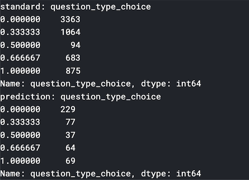\n\nIn the following image, I was trying to mark which columns I need to do fine-tuning. The horizontal yellow lines indicated that I didn't need to do too much about those columns. The scores like 0.5 and 1.0 in other graphs indicated that I need to do some extra thresholding at those values. \n\n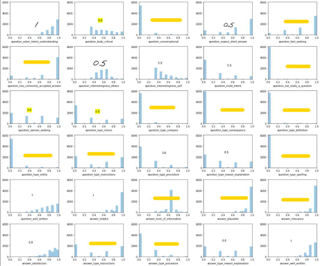\n\n\n\n##Update Technical Part:\n\n### **Feature Engineering:**\nInspired by pubic kernels, we extract URLs from the *url* column and implemented one-hot\nencoding to both the URLs and category columns. There are 64 new feature columns (51 for\n*url* and 13 for *category*) after one-hot encoding. According to the paper *Universal Sentence\nEncoder*, The Universal Sentence Encoder (USE) encodes text into high dimensional vectors\nthat can be used for diverse tasks. The input is the variable-length English text, and the output\nis a 512-dimensional vector. So, we encoded question title, question body, and answer into\n512-dimensional vectors and then compared the L2 distance and cosine similarities between\nthem. We then added all of these as new features. There are 512 + 512 + 64 + 2 = 1090 new\nfeatures.\nUnder the concern of overfitting, I tried to decrease the number of generated features by\nbriefly reading through a few examples of each category and then manually reclassifying 51\ncategories into four sub-categories: *have code, daily life, academic, literature readings*.\nHowever, this didn’t improve the prediction.\n\n\n###**Model Structure:**\nWe used a combo of two pretrained Roberta base models to train the dataset. The first\nRoberta handles the question title and question body pairs, while the second Roberta handles\nthe question title and answer pairs. We only fitted texts into Roberta models and ignored\n1090 new features for now.\nThe Roberta base model has 12 hidden layers and there are 13 layers in total (which includes\nthe final output layer). Every layer has the output dimension *batch_size* x 512 x 768 (*batch\n_size x max_seq_len x emb_size*). Initially, I tried out convolutions with different filter sizes\nsuch as 4 x 768, 6 x 768 or 8 x 768 to capture the meaning of the combination of words.\nHowever, it turned out to not work that well, and the average of the whole sequences\noutperformed them.\nWe took the last three output layers out, concatenated them together and then applied an\naverage-pooling on it. After this, we averaged over 512 tokens for each input in the batch to\ncapture the meaning of the whole sequence and hoped the model would learn some lower\nlevel features and added them to the final representation. Finally, we concatenated 1090\nfeatures with the average embedding and then added a fully connected layer with 21 units for\nthe title-body pair model and 9 units for the title-answer pair model.\nI didn’t use the first unit of the output layer of the Roberta model since Roberta removes the\n*Next Sentence Prediction (NSP)* task from BERT’s pre-training, and the first unit seems not\nas useful as in Bert. The final predictions are the average of 6 pairs of Roberta models (6-\nfold).\nWe were supposed to freeze Roberta models and then fine-tune the added fully connected\nlayer, but we didn’t due to the time limit.\n\n\n###**Customized Learning rate:**\nWe used a range test in the beginning, to find out the proper learning rate during training. We\nthen wrote up a customized scheduler inherited from PolynomialDecay to change the\nlearning rate dynamically. We set up warm-up steps proportional to the total decay-steps to\navoid the primacy effect at the beginning of the training process. The learning rate increases\nlinearly over the warm-up period and we didn’t set up the learning rate to have cyclic\nbehavior.\n\n\n###**Training:**\nLike most of the other groups, we use GroupKFold with n_splits=5, did 6-fold cv for 6\nepochs and saved the training weights with the highest cv scores. We used Adam optimizer\nwith mixed-precision data types, which dynamically and automatically adjusting the scaling\nto prevent Inf or NaN values and saved training time.\n\n\n###**Post-processing:**\nWe first considered using one-hot encoding for all output columns, given that every column\nhas finite discrete values, but this shouldn’t work well since it didn’t take the order of the\nvalues into account. Because of the time limit, we just compared the distribution of\npredictions for each column with the distribution of actual values in the training set and then\nadjust the threshold based on the distribution. We compared the scores between before post-\nprocessing and after post-processing to see if it improved performance.", "votes": 16 }, { "id": 1041953, "postDate": "2020-10-08T01:45:55.240Z", "content": "Hope to try the Roberta
", "rawMarkdown": "Hope to try the Roberta" }, { "id": 1037861, "postDate": "2020-10-05T11:55:05.747Z", "content": "Congrats! Can I ask if i set up the learning rate to have cyclic
\nbehavior,Will it mess up?
Thank You for the solution. I have a question, how did you decide what labels to fine tune and what labels not to fine tune? Is it because the plots with horizontal yellow line have less discrete values ?
", "rawMarkdown": "Thank You for the solution. I have a question, how did you decide what labels to fine tune and what labels not to fine tune? Is it because the plots with horizontal yellow line have less discrete values ? " }, { "id": 752511, "postDate": "2020-02-21T05:21:02.287Z", "content": "Discussion updated.
", "rawMarkdown": "Discussion updated." }, { "id": 743058, "postDate": "2020-02-11T18:45:48.890Z", "content": "Congrats!
", "rawMarkdown": "Congrats! " }, { "id": 742247, "postDate": "2020-02-11T07:24:02.903Z", "content": "Nice solution and congrats ! Can I ask how exactly you moved the models predicted score towards a score that \"made sense\" ?
", "rawMarkdown": "Nice solution and congrats ! Can I ask how exactly you moved the models predicted score towards a score that \"made sense\" ?", "replies": [ { "id": 742279, "postDate": "2020-02-11T07:48:57.457Z", "content": "Hi, this is how I do it.\npython\ndef closest(num_list, num): \nBut be careful. Some columns have a unique value after I did this modification. You need to find it and manully design a threshold so that the column values are not unique. Otherwise, you will get a submission error. It frustrated me a lot but I finally figured it out by checking the discussion.
\n '''\n num_list is an array of all values of the corresponding last 30 columns in the training set. \n '''\n idx = (np.abs(num_list - num)).argmin() \n return num_list[idx]\n
Aah. I see. Thanks a lot for the reply :)
", "rawMarkdown": "Aah. I see. Thanks a lot for the reply :) " } ] }, { "id": 742980, "postDate": "2020-02-11T17:17:42.453Z", "rawMarkdown": "", "isDeleted": true } ], "complete": true, "source": "live", "fetched_at": "2026-10-19T19:07:47Z", "competition_id": 7968, "competition_slug": "google-quest-challenge", "team_id": 4318804, "solution_url": "/competitions/google-quest-challenge/writeups/lytang-a-general-walk-through-my-solution-with-tri" }